Table of content
Adjustable robust optimization with discrete uncertainty > DisruptionFLP
gap = function(LB, UB) {
  return(100 * abs(LB - UB) / (1e-10 + abs(UB)))
}
key = c("instance", "gamma")
time_limit = 3600raw_benders = read.csv("./results_benders_DisruptionFLP.csv", header = FALSE)
colnames(raw_benders) <- c("instance", "gamma", "status", "reason", "objective", "time", "nodes", "rel_gap", "abs_gap", "n_generated_cuts")
paged_table(raw_benders)Unifying format
To make our study easier, we start by unifying the format of each dataset. To do so, we transform our data to obtain it in the following format:
- instance: the instance filename ;
- n_facilities: the number of facilities ;
- n_customers: the number of customers ;
- gamma: the value of \(\Gamma\) ;
- objective: the best objective value found (feasible) ;
- time: the computation time spent solving the instance.
We thus introduce two functions read_csv_benders and
read_csv_ccg which first reads an input file for the
corresponding approach and returns the associated formatted table.
Before that, we first introduce a helper function
parse_instance_properties which takes a list of instances
as input and returns a table containing, for each instance, the number
of knapsacks, the number of items and the value for alpha extracted from
the instance file name.
library(stringr)

parse_instance_properties = function (instances) {

  parsed = t(apply(as.matrix(instances), 1, function(str)  str_extract_all(str, regex("([0-9]+)"))[[1]]))

  result = data.frame(instances, as.double(parsed[,1]), as.double(parsed[,2]), as.double(parsed[,3]))
  colnames(result) = c("instance", "n_facilities", "n_customers", "ratio")

  return (result)

}
read_csv_benders
The `read_csv_benders`` function is given as follows.
read_csv_benders = function(filename) {

  # Read raw results
  raw_results = read.csv(filename, header = FALSE)
  colnames(raw_results) <- c("instance", "gamma", "status", "reason", "objective", "time", "nodes", "rel_gap", "abs_gap", "n_generated_cuts")

  # Fix unsolved instances to TIME_LIMIT
  if (sum(raw_results$time >= 3600) > 0) {
    raw_results[raw_results$time >= 3600,]$time = 3600
  }

  # Extract properties from instance file names
  properties = parse_instance_properties(raw_results$instance)

  # Build result data frame
  result = data.frame(
      properties$instance,
      properties$n_facilities,
      properties$n_customers,
      properties$ratio,
      raw_results$gamma,
      raw_results$objective,
      raw_results$time,
      raw_results$nodes,
      raw_results$rel_gap * 100,
      "B&C"
    )
  colnames(result) = c("instance", "n_facilities", "n_customers", "ratio", "gamma", "objective", "time", "nodes", "gap", "solver")

  result = result[result$ratio != 150,]

  return (result)

}
We can then read CSV files coming from the benders approach.
benders = read_csv_benders("./results_benders_DisruptionFLP.csv")read_csv_ccg
The `read_csv_ccg`` function is given as follows.
read_csv_ccg = function (filename) {

  # Read raw results
  raw_results = read.csv(filename, header = FALSE)
  colnames(raw_results) <- c("instance", "gamma", "iter", "LB", "UB", "time", "inner_iter_1", "inner_iter_2")

  # Fix unsolved instances to TIME_LIMIT
  if (sum(raw_results$time >= 3600) > 0) {
    raw_results[raw_results$time >= 3600,]$time <- 3600
  }

  # Extract properties from instance file names
  properties = parse_instance_properties(raw_results$instance)

  # Build result data frame
  result = data.frame(
      properties$instance,
      properties$n_facilities,
      properties$n_customers,
      properties$ratio,
      raw_results$gamma,
      raw_results$UB,
      raw_results$time,
      NA,
      gap(raw_results$LB, raw_results$UB),
      "CCG"
    )
  colnames(result) = c("instance", "n_facilities", "n_customers", "ratio", "gamma", "objective", "time", "nodes", "gap", "solver")

  raw_results[abs(raw_results$UB) < 1e-6 & abs(raw_results$LB) < 1e-6,]$gap = 0

  result = result[result$ratio != 150,]

  return (result)

}
Then, we read the results obtained by the CCG approach as follows.
ccg = read_csv_ccg("./results_ccg_DisruptionFLP.csv")## Warning in `[<-.data.frame`(`*tmp*`, abs(raw_results$UB) < 0.000001 &
## abs(raw_results$LB) < : provided 11 variables to replace 10 variablesChecking
compare = function(a, b) {
  A = a[a$time < 3600,c("instance", "gamma", "objective", "time")]
  B = b[b$time < 3600,c("instance", "gamma", "objective", "time")]

  merged = merge(A, B, by = c("instance", "gamma"))

  filter = gap(merged$objective.x, merged$objective.y) > 1e-3
  if (sum( filter ) > 0) {
    print("For some instances, the two methods do not agree.")
    paged_table( merged[filter,] )
  }
}

compare(benders, ccg)
Performance profile
all_results = rbind(benders, ccg)

solvers = unique(all_results$solver)

colors = cbind(as.data.frame(solvers), rainbow(length(solvers)))
colnames(colors) = c("solver", "color")
performance_profile = function (dataset, xlim = NULL, main = "Performance profile") {
times = spread(dataset[,c("instance", "gamma", "solver", "time")], key = solver, value = time)
times$time.best = apply(times[,-c(1,2)], 1, FUN = min)
#times = na.omit(times)
#print("WARNING omitting NA")
ratios = times[,-ncol(times)][,-c(1,2)] / times$time.best
colnames(ratios) = paste0(colnames(ratios), ".ratio")
worst_ratio = max(ratios)
times = cbind(times, ratios)
for (solver in solvers) {
time_limit_filter = times[,solver] >= time_limit
if ( sum(time_limit_filter) > 0 ) {
times[time_limit_filter, paste0(solver, ".ratio")] = worst_ratio
}
}
if (is.null(xlim)) {
xlim = c(1, worst_ratio)
}
#par(mar = c(5,4,4,8))
using_colors = NULL
using_types = NULL
last_ecdf = NULL
index = 1
for (solver in solvers) {
plot_function = if (index == 1) plot else lines
profile = ecdf(times[,paste0(solver, ".ratio")])
using_color = colors[colors$solver == solver,2]
using_colors = rbind(using_colors, using_color)
using_type = "solid"
if (using_color == "#00FFFFFF") {
using_type = "dashed"
}
using_types = rbind(using_types, using_type)
plot_function(profile, xlim = xlim, ylim = c(0,1), lty = using_type, cex = 0, col = using_color, main = "", xlab = "", ylab = "")
if (is.null(last_ecdf)) {
last_ecdf = profile
} else {
p = seq(0, 1, length.out = 50000)
df = data.frame(
quantile(last_ecdf, probs = p),
quantile(profile, probs = p)
)
colnames(df) = solvers
print( head( df[df["CCG"] > df["B&C"],], 1 ))
}
index = index + 1
}
# Set the plot title
title(main = main,
xlab = "Performance ratio",
ylab = "ECDF")
# Set the plot legend
legend(
"bottomright",
#inset=c(-.35, 0),
legend = solvers,
lty = using_types,
col = using_colors,
#cex = .5,
#xpd = TRUE,
bty = "n"
)
}{
performance_profile(all_results)
performance_profile(all_results, xlim = c(1, 100), main = "Performance profile")
}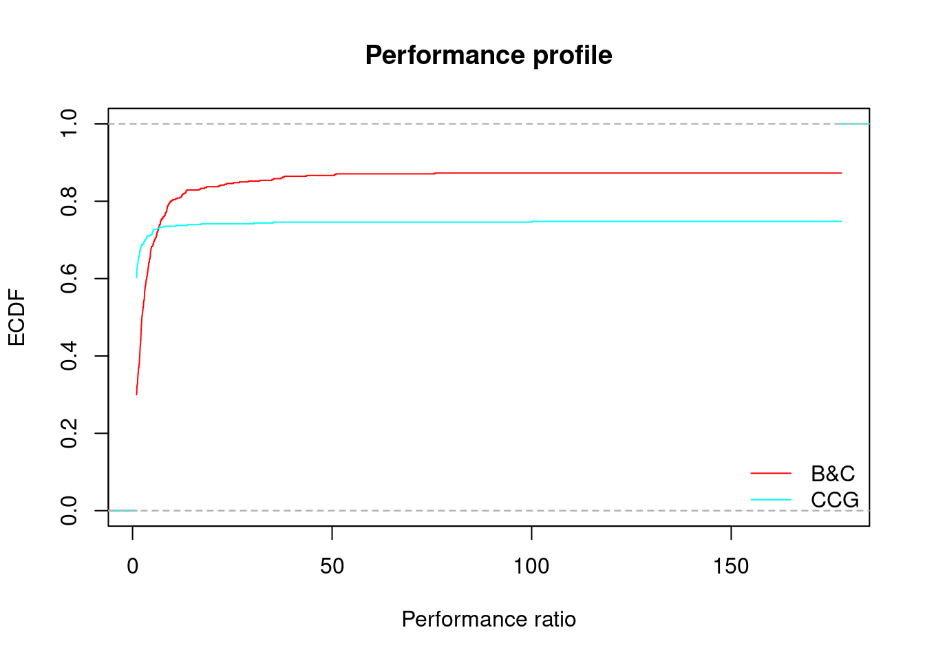
##                   B&C     CCG
## 72.99145983% 6.533554 6.53648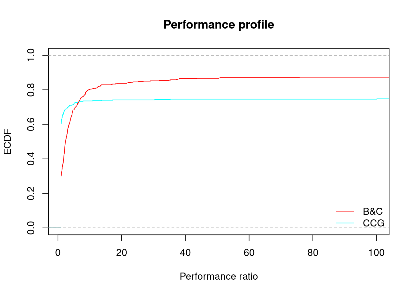
##                   B&C     CCG
## 72.99145983% 6.533554 6.53648
#for (gamma in unique(all_results$gamma)) {
# performance_profile(all_results[all_results$gamma == gamma,], main = paste("With gamma =", gamma))
#}
for (ratio in unique(all_results$ratio)) {
performance_profile(all_results[all_results$ratio == ratio,], xlim = c(1, 70), main = "")
}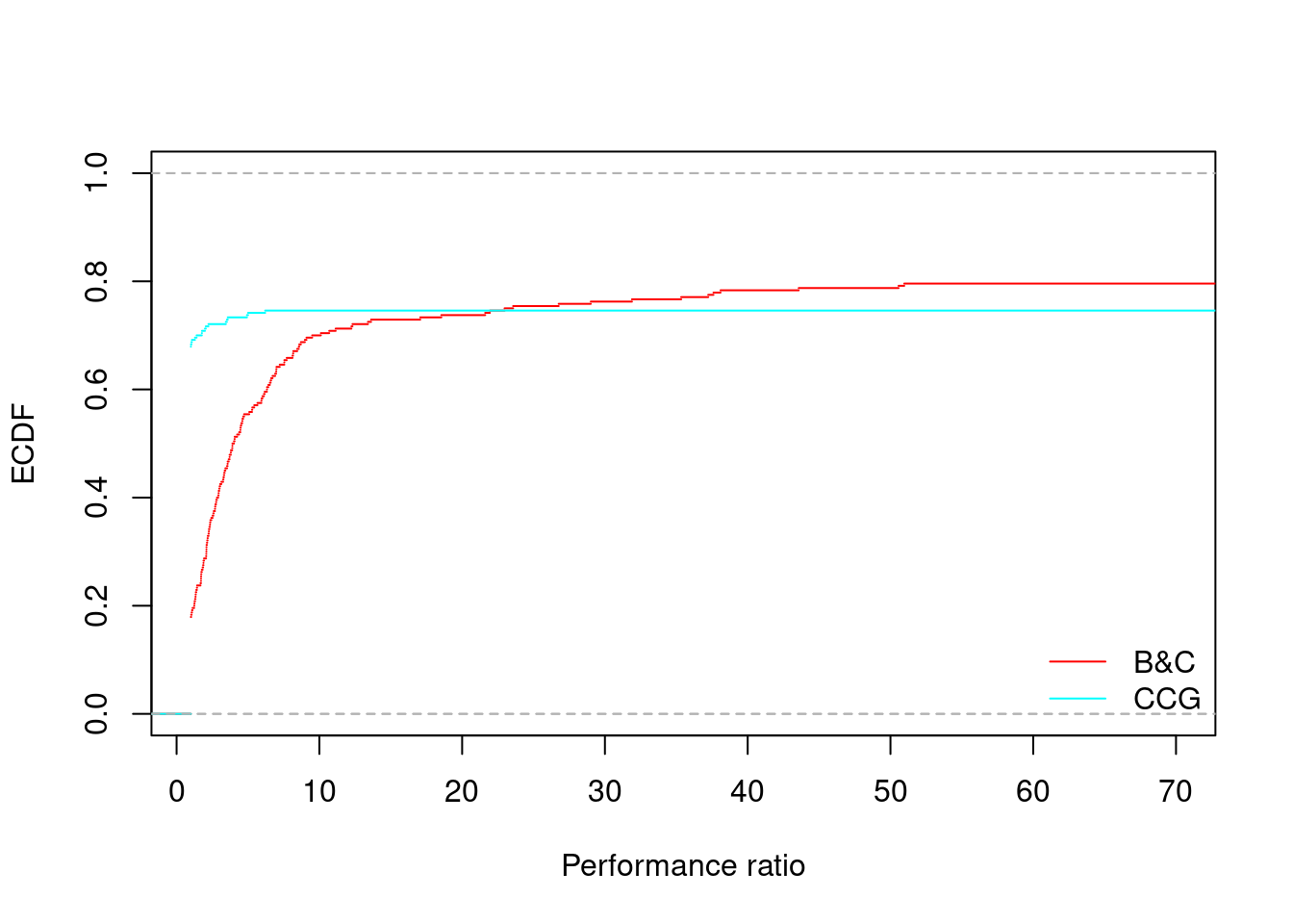
##                   B&C      CCG
## 74.57349147% 22.18092 22.24441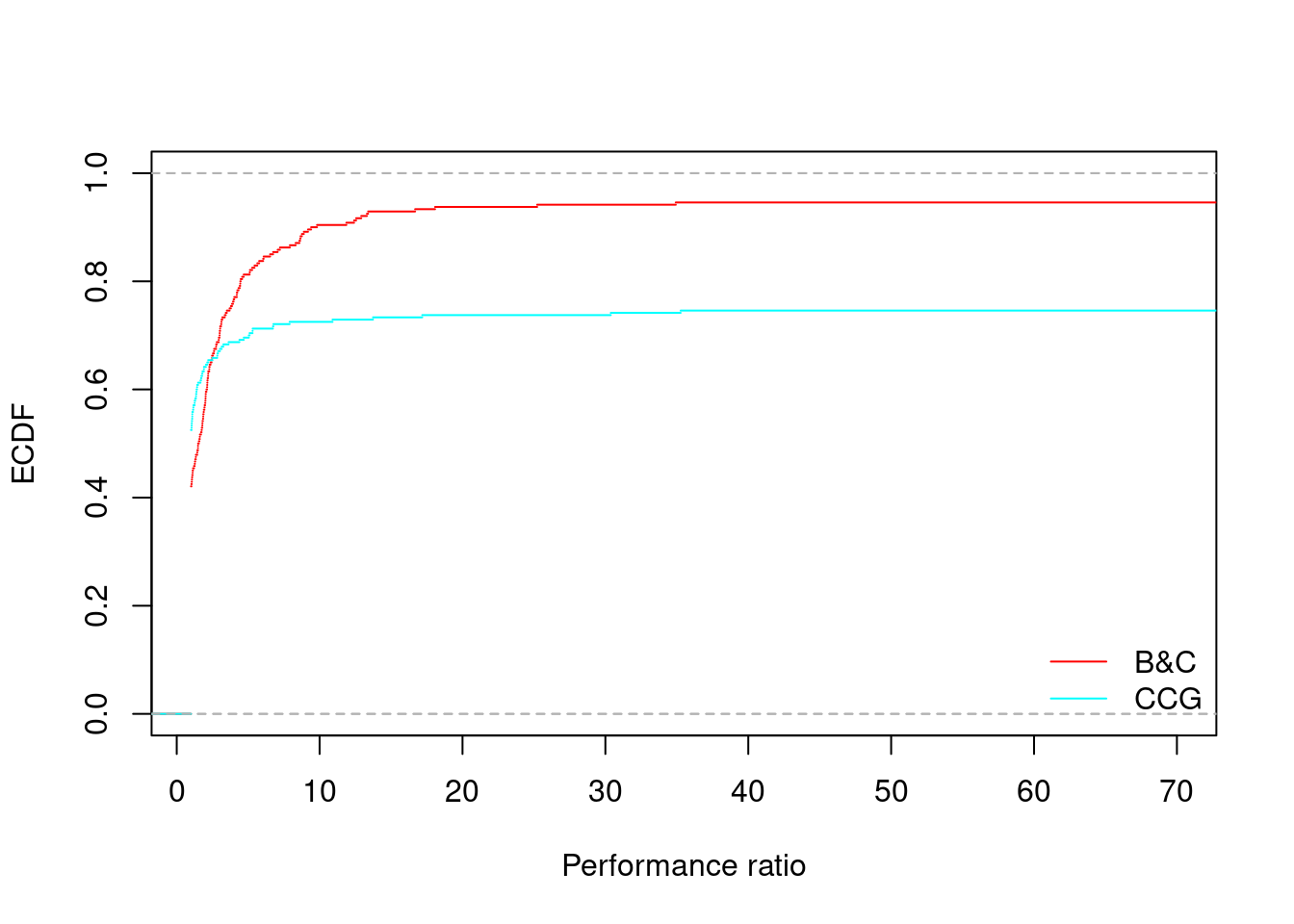
##                   B&C      CCG
## 65.64931299% 2.468363 2.469409
Summary tables
group_by = c("ratio", "gamma", "n_facilities", "n_customers")
str_group_by = c("$\\mu$", "$\\Gamma$", "$|V_1|$", "$|V_2|$")
Computing summary times by group
We start by calling summary on each group. This will
compute, for each group, the minimum, 1st quantile, median, mean, 3rd
quantile and maximum execution time. This is done in the following
function which takes as parameter the formatted table with all
results.
compute_summary_by_group = function(data) {

  # We summarize only the solved instances
  data = data[data$time < 3600,]

  # We aggregate by `group_by` using `summary`
  result = aggregate(data$time, by = data[,group_by], summary)

  # Here, we call data.frame recursively to flatten `result` (summary does create a nested structure)
  result = do.call(data.frame, result)

  # Then, we set column names
  colnames(result) = c(group_by, "min", "1st_quantile", "median", "mean", "3rd_quantile", "max")

  return (result)
}
We then call this function on each approach.
summary_ccg = compute_summary_by_group(ccg)
summary_benders = compute_summary_by_group(benders)
Computing number of solved instances by group
We then count the number of instances which could not be solved to optimality within each group. This is done in the following function.
compute_solved_by_group = function(data) {

  # Aggregate groups using `sum` over the filter returning 1 iff the time limit is reached
  result = aggregate(data$time < 3600, by = data[,group_by], sum)

  # Set column and row names
  colnames(result) = c(group_by, "solved")
  rownames(result) = NULL

  return (result)

}
Again, we call this function on each approach.
solved_ccg = compute_solved_by_group(ccg)
solved_benders = compute_solved_by_group(benders)
Computing average gap of unsolved instances by group
We then compute the average final gap over those instances which could not be solved to optimality within each group. This is done in the following function.
compute_gap_by_group = function(data) {

  # Aggregate groups using `sum` over the filter returning 1 iff the time limit is reached
  result = aggregate(data$gap, by = data[,group_by], mean)

  # Set column and row names
  colnames(result) = c(group_by, "gap")
  rownames(result) = NULL

  return (result)

}
Again, we call this function on each approach.
gap_ccg = compute_gap_by_group(ccg)
gap_benders = compute_gap_by_group(benders)
Computing average number of nodes instances by group
We then compute the average final gap over those instances which could not be solved to optimality within each group. This is done in the following function.
compute_nodes_by_group = function(data) {

  only_solved = data[data$time < 3600,]

  # Aggregate groups using `sum` over the filter returning 1 iff the time limit is reached
  result = aggregate(only_solved$node, by = only_solved[,group_by], mean)

  # Set column and row names
  colnames(result) = c(group_by, "node")
  rownames(result) = NULL

  return (result)

}
Again, we call this function on each approach.
nodes_ccg = compute_nodes_by_group(ccg)
nodes_benders = compute_nodes_by_group(benders)
Computing number of instances by group
Finally, we also count the number of instances which was tried by each approach. (Note that when experiments are done, they should all be equal).
compute_instances_by_group = function(data) {

  # Call length on each group to count the number of instances
  result = aggregate(data$instance, by = data[,group_by], length)

  # Set row and column names
  colnames(result) = c(group_by, "total")
  rownames(result) = NULL

  return (result)

}
Let’s call it on each approach.
total_ccg = compute_instances_by_group(ccg)
total_benders = compute_instances_by_group(benders)
Summary table
Final result
We are now ready to build our summary table. In what follows, we
introduce a helper function to add the useful columns of a by-group
result (i.e., total_<APPROACH>,
unsolved_<APPROACH> or
summary_<APPROACH>) to the main table, called
Table.
# Helper function
add_columns = function(table, data, suffix) {
  result = merge(table, data, by = group_by, all = TRUE, suffixes = c("", paste(".", suffix, sep = "")))
  return (result)
}

# We list the useful columns of the by-group results
column_names = c("total", "solved", "min", "1st_quantile", "median", "mean", "3rd_quantile", "max", "gap", "node")

# We create an empty data frame with column names. This is used to
# (1) create the placeholder for the group identifiers
# (2) force R to rename each added column by appending a suffix to it
Table = data.frame(matrix(ncol = length(group_by) + length(column_names), nrow = 0))
colnames(Table) = c(group_by, column_names)

# We add by-group totals
Table = add_columns(Table, total_benders, "B&C")
Table = add_columns(Table, total_ccg, "CCG")

# We add by-group solved
Table = add_columns(Table, solved_benders, "B&C")
Table = add_columns(Table, solved_ccg, "CCG")

# We add by-group summaries
Table = add_columns(Table, summary_benders, "B&C")
Table = add_columns(Table, summary_ccg, "CCG")

# We add by-group gap
Table = add_columns(Table, gap_benders, "B&C")
Table = add_columns(Table, gap_ccg, "CCG")

# We add by-group gap
Table = add_columns(Table, nodes_benders, "B&C")

# Finally, we can remove the "fake" columns we introduced to foce R renaming new columns
Table = Table[,!names(Table) %in% column_names]
The resulting table therefore contains a merge of all by-group data and is drawn hereafter.
To better summarize our data, we make a new table out of this table by selecting interesting columns. This is done as follows.
Table1 = Table[,c(
  group_by,
  "solved.B&C",
  "solved.CCG",
  "mean.B&C",
  "mean.CCG",
  "gap.B&C",
  "gap.CCG",
  "node.B&C"
)]|
Solved
|
Time
|
Gap
|
Node
|
|||||||
|---|---|---|---|---|---|---|---|---|---|---|
| \(\mu\) | \(\Gamma\) | \(&#124;V_1&#124;\) | \(&#124;V_2&#124;\) | B&C | CCG | B&C | CCG | B&C | CCG | B&C |
| 200 | 2 | 10 | 20 | 10 | 10 | 13.61 | 4.98 | 0.00 | 0.00 | 19 |
| 200 | 2 | 10 | 30 | 10 | 10 | 64.50 | 106.81 | 0.00 | 10.00 | 36 |
| 200 | 2 | 10 | 40 | 10 | 8 | 254.90 | 40.25 | 0.00 | 7.95 | 27 |
| 200 | 2 | 10 | 50 | 10 | 10 | 1058.59 | 106.21 | 0.00 | 0.00 | 30 |
| 200 | 2 | 15 | 20 | 10 | 9 | 122.09 | 134.87 | 0.00 | 12.46 | 63 |
| 200 | 2 | 15 | 30 | 10 | 6 | 742.82 | 553.81 | 0.00 | 5.19 | 60 |
| 200 | 2 | 15 | 40 | 6 | 7 | 1509.53 | 92.54 | 1.93 | 4.96 | 82 |
| 200 | 2 | 15 | 50 | 5 | 6 | 1882.22 | 560.80 | 2.70 | 5.93 | 50 |
| 200 | 3 | 10 | 20 | 10 | 10 | 22.74 | 8.46 | 0.00 | 30.91 | 31 |
| 200 | 3 | 10 | 30 | 10 | 10 | 75.81 | 37.17 | 0.00 | 0.00 | 38 |
| 200 | 3 | 10 | 40 | 10 | 10 | 213.18 | 95.80 | 0.00 | 20.00 | 36 |
| 200 | 3 | 10 | 50 | 8 | 8 | 658.77 | 451.47 | 27.12 | 2.04 | 34 |
| 200 | 3 | 15 | 20 | 10 | 7 | 218.62 | 69.42 | 0.00 | 32.40 | 88 |
| 200 | 3 | 15 | 30 | 10 | 4 | 1320.35 | 177.90 | 0.00 | 19.18 | 55 |
| 200 | 3 | 15 | 40 | 4 | 7 | 1353.41 | 468.41 | 5.55 | 2.57 | 58 |
| 200 | 3 | 15 | 50 | 1 | 3 | 3572.38 | 856.32 | 8.89 | 39.34 | 51 |
| 200 | 4 | 10 | 20 | 10 | 10 | 34.25 | 3.38 | 0.00 | 30.01 | 84 |
| 200 | 4 | 10 | 30 | 10 | 10 | 121.93 | 37.88 | 0.00 | 25.94 | 162 |
| 200 | 4 | 10 | 40 | 10 | 10 | 360.44 | 198.41 | 0.00 | 72.07 | 165 |
| 200 | 4 | 10 | 50 | 8 | 9 | 1000.25 | 306.56 | 7.72 | 14.66 | 107 |
| 200 | 4 | 15 | 20 | 10 | 6 | 452.02 | 246.01 | 0.00 | 9985652759414.99 | 496 |
| 200 | 4 | 15 | 30 | 7 | 3 | 806.49 | 147.91 | 13.49 | 13452069676498.95 | 72 |
| 200 | 4 | 15 | 40 | 3 | 4 | 1210.74 | 1280.90 | 7.00 | 13.95 | 78 |
| 200 | 4 | 15 | 50 | 0 | 2 | NA | 1241.74 | 39.03 | 108.12 | NA |
| 300 | 2 | 10 | 20 | 10 | 10 | 13.42 | 12.83 | 0.00 | 0.00 | 47 |
| 300 | 2 | 10 | 30 | 10 | 9 | 18.50 | 251.17 | 0.00 | 1.98 | 32 |
| 300 | 2 | 10 | 40 | 10 | 10 | 15.92 | 70.54 | 0.00 | 0.00 | 30 |
| 300 | 2 | 10 | 50 | 10 | 7 | 158.93 | 94.25 | 0.00 | 19.77 | 47 |
| 300 | 2 | 15 | 20 | 10 | 9 | 69.06 | 110.83 | 0.00 | 2.42 | 72 |
| 300 | 2 | 15 | 30 | 10 | 7 | 102.49 | 406.04 | 0.00 | 9.19 | 33 |
| 300 | 2 | 15 | 40 | 9 | 5 | 324.90 | 142.36 | 0.07 | 13.47 | 87 |
| 300 | 2 | 15 | 50 | 10 | 9 | 250.11 | 445.83 | 0.00 | 4.72 | 45 |
| 300 | 3 | 10 | 20 | 10 | 9 | 29.79 | 37.91 | 0.00 | 14295287681237.00 | 99 |
| 300 | 3 | 10 | 30 | 10 | 10 | 104.54 | 49.70 | 0.00 | 0.00 | 80 |
| 300 | 3 | 10 | 40 | 10 | 10 | 45.13 | 36.49 | 0.00 | 10.00 | 65 |
| 300 | 3 | 10 | 50 | 10 | 7 | 230.14 | 254.23 | 0.00 | 62.61 | 66 |
| 300 | 3 | 15 | 20 | 10 | 8 | 126.99 | 109.51 | 0.00 | 5.53 | 89 |
| 300 | 3 | 15 | 30 | 10 | 6 | 359.67 | 264.51 | 0.00 | 16.85 | 60 |
| 300 | 3 | 15 | 40 | 9 | 2 | 1093.62 | 190.89 | 0.85 | 23.41 | 100 |
| 300 | 3 | 15 | 50 | 10 | 6 | 908.34 | 768.34 | 0.00 | 13.62 | 65 |
| 300 | 4 | 10 | 20 | 10 | 10 | 41.74 | 7.63 | 0.00 | 7.10 | 227 |
| 300 | 4 | 10 | 30 | 10 | 10 | 185.98 | 31.53 | 0.00 | 40.08 | 380 |
| 300 | 4 | 10 | 40 | 10 | 10 | 56.94 | 18.36 | 0.00 | 10.00 | 110 |
| 300 | 4 | 10 | 50 | 10 | 8 | 607.93 | 610.69 | 0.00 | 2.16 | 117 |
| 300 | 4 | 15 | 20 | 10 | 9 | 376.20 | 576.29 | 0.00 | 2.47 | 675 |
| 300 | 4 | 15 | 30 | 10 | 5 | 1195.95 | 182.24 | 0.00 | 63.28 | 207 |
| 300 | 4 | 15 | 40 | 5 | 2 | 1875.86 | 562.71 | 11.97 | 30.50 | 113 |
| 300 | 4 | 15 | 50 | 4 | 2 | 1190.49 | 704.55 | 21.23 | 41.09 | 77 |
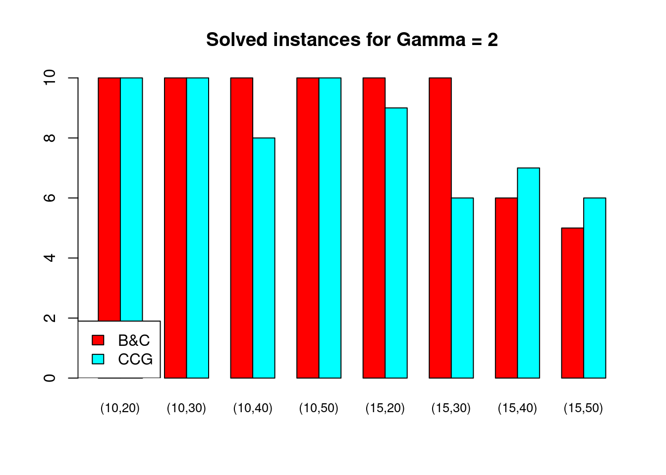
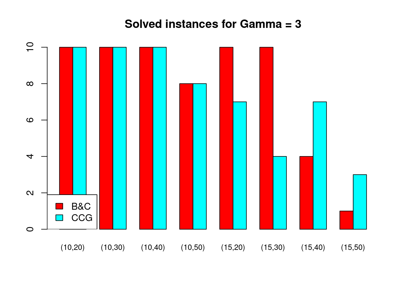
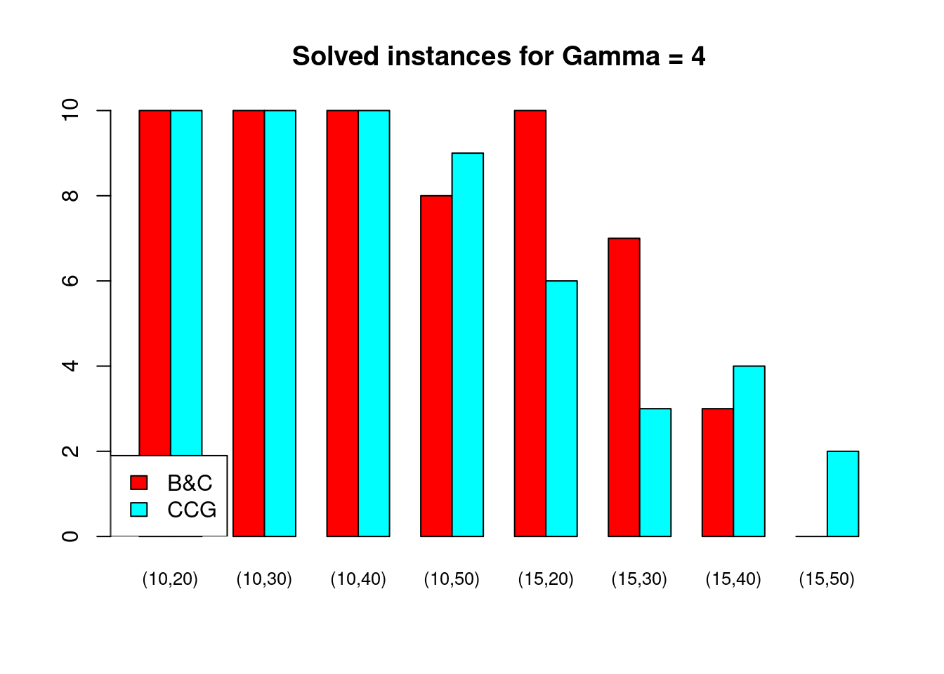
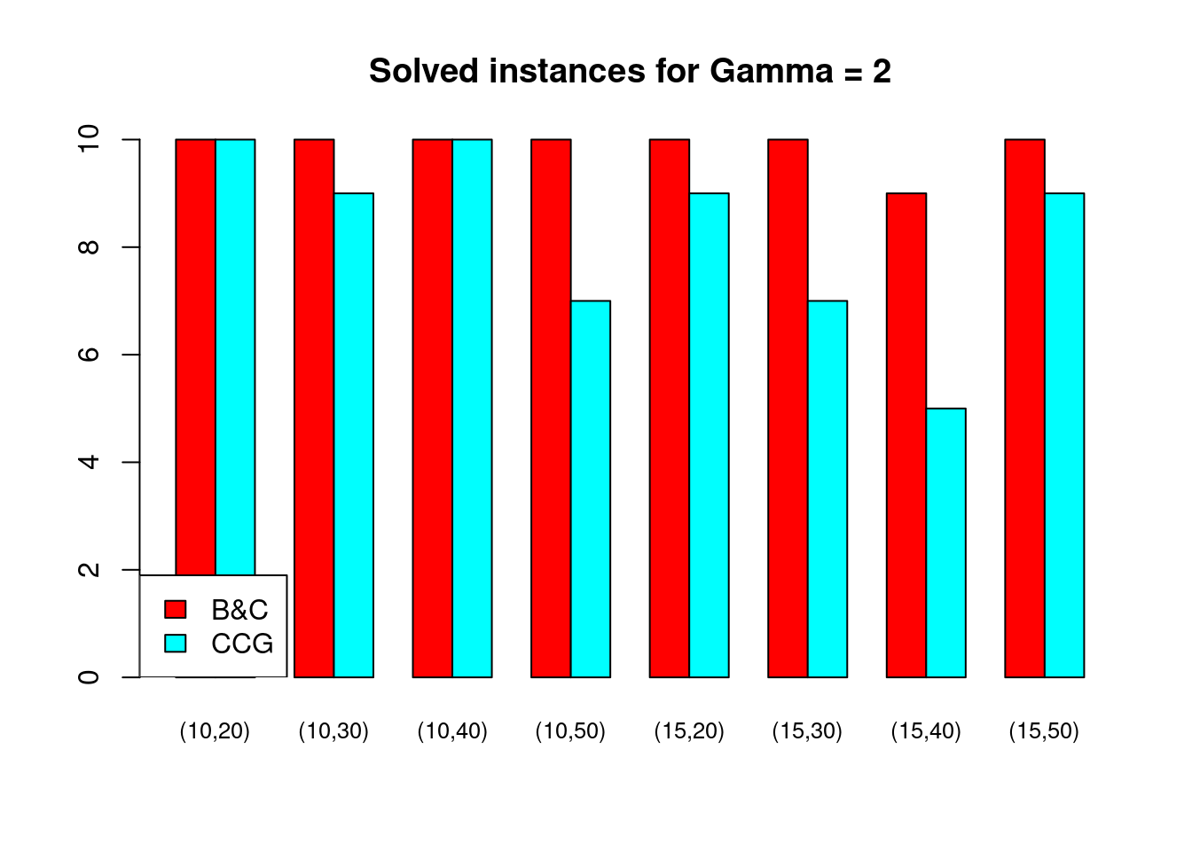
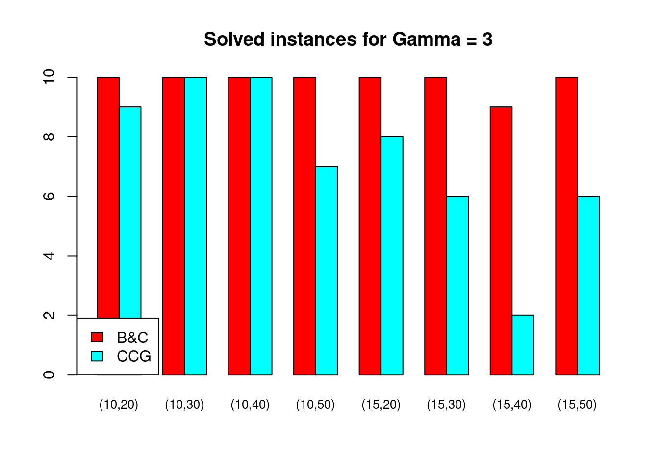
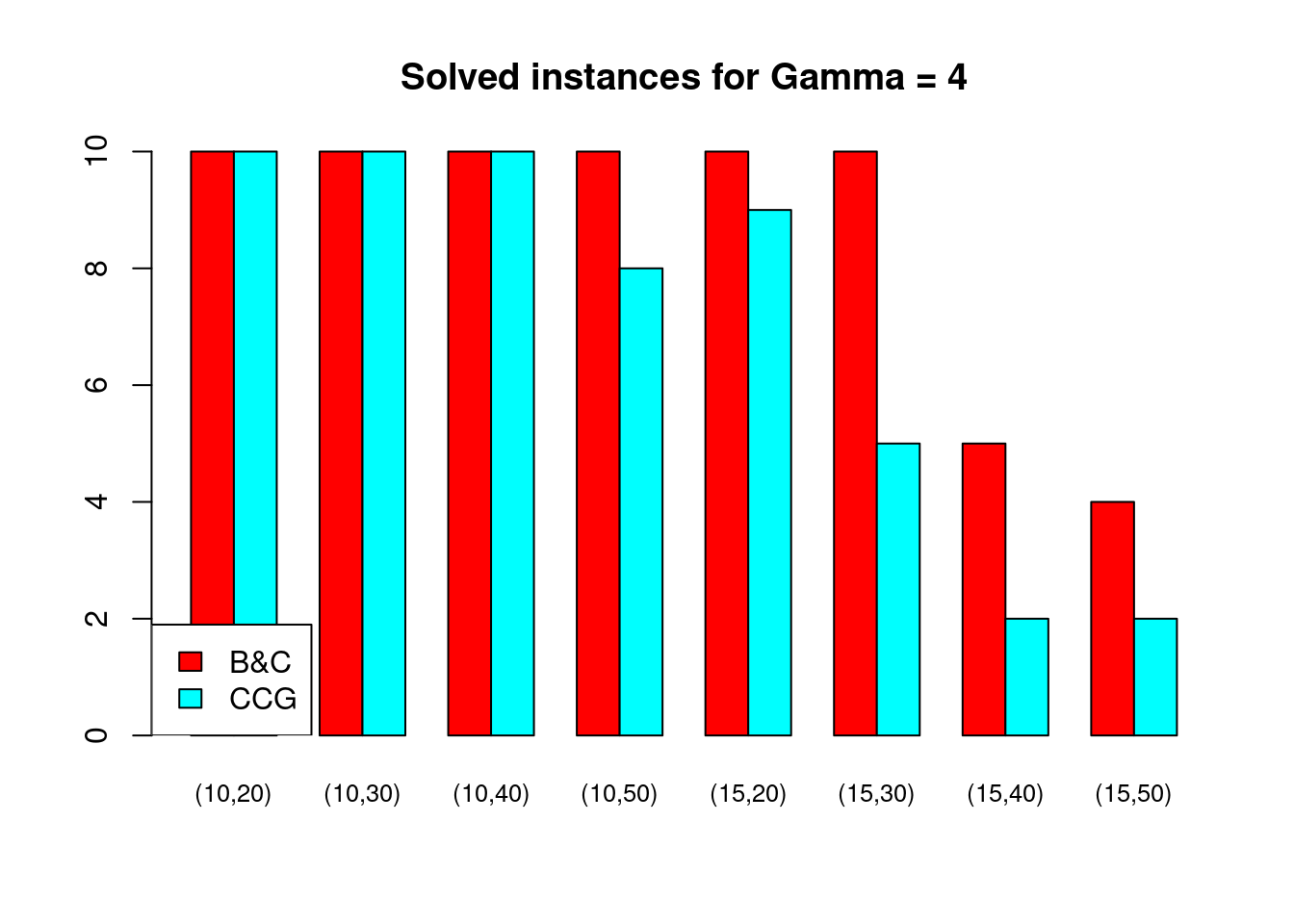
Solved instances
plot_solved = function (dataset, main = "Solved instances") {
  data = dataset[, c("solved.B&C", "solved.CCG")]
  rownames(data) = paste0("(", dataset$n_facilities, ",", dataset$n_customers, ")")
  data = t(as.matrix(data))
  barplot( data , beside = TRUE, col = colors$color, main = main, ylim = c(0, 10), cex.names=.8)
  legend("bottomleft",  legend = c("B&C", "CCG"), fill = colors$color)
}
for (ratio in unique(Table$ratio)) {
for (gamma in unique(Table$gamma)) {
plot_solved(Table[Table$gamma == gamma & Table$ratio == ratio,], main = paste("Solved instances for Gamma =", gamma))
}
}
Partial disruptions (\(K > 1\))
In this section, we study how B&C performs when increasing the number of unknown coefficients. This leads to the partial disruption FLP application (Note that \(K\) has been replaced by \(R\) in the paper).
We start by parsing the results stored in the “./resutls_PartialDisruptionFLP.csv” file.
read_csv_benders_partial = function(filename) {

  # Read raw results
  raw_results = read.csv(filename, header = FALSE)
  colnames(raw_results) <- c("instance", "gamma", "status", "reason", "objective", "time", "nodes", "LB", "UB", "n_generated_cuts", "k")

  # Fix unsolved instances to TIME_LIMIT
  if (sum(raw_results$time >= 3600) > 0) {
    raw_results[raw_results$time >= 3600,]$time = 3600
  }

  # Extract properties from instance file names
  properties = parse_instance_properties(raw_results$instance)

  # Build result data frame
  result = data.frame(
      properties$instance,
      properties$n_facilities,
      properties$n_customers,
      properties$ratio,
      raw_results$gamma,
      raw_results$objective,
      raw_results$time,
      raw_results$nodes,
      "B&C",
      raw_results$k
    )
  colnames(result) = c("instance", "n_facilities", "n_customers", "ratio", "gamma", "objective", "time", "nodes", "solver", "k")

  return (result)

}

raw_benders_partial = read_csv_benders_partial("./results_PartialDisruptionFLP.csv")
Then, we transform these raw data to obtain, for each instance, the computational time required to solve the instance for different values of \(K\).
by_k = spread(raw_benders_partial[, c("instance", "n_facilities", "n_customers", "ratio", "gamma", "time", "k")], key = k, value = time)
rownames(by_k) = NULL
Then, we first make sure that each instance have been solved for
\(K = 1, 2, 3\) and \(4\) by printing rows where NA
appear.
paged_table(by_k[!complete.cases(by_k),])Median computation times
by_k = na.omit(by_k)
partial_mean = aggregate(by_k[,c("1", "2", "3", "4")], by = by_k[,c("n_facilities", "n_customers", "gamma")], median)|
Median time
|
||||||
|---|---|---|---|---|---|---|
| \(&#124;V_1&#124;\) | \(&#124;V_2&#124;\) | \(\Gamma\) | 1 | 2 | 3 | 4 |
| 10 | 20 | 2 | 13.39 | 45.74 | 96.05 | 164.51 |
| 15 | 20 | 2 | 65.77 | 212.10 | 573.99 | 1404.95 |
| 10 | 30 | 2 | 14.91 | 64.47 | 139.69 | 283.84 |
| 15 | 30 | 2 | 123.60 | 620.90 | 1886.20 | 3600.00 |
| 10 | 40 | 2 | 17.57 | 66.29 | 220.63 | 506.31 |
| 10 | 50 | 2 | 41.43 | 500.92 | 1529.26 | 3233.98 |
Graphical representation
plot_evolution = function(dataset, main = "Evolution of computational times depending on K") {

  #dataset$type = paste0("(", dataset$n_facilities, ",", dataset$n_customers, "), Gamma = ", dataset$gamma)
  dataset$type = paste0("(", dataset$n_facilities, ",", dataset$n_customers, ")")

  #longest = max(dataset[ ,"4"])

  longest = 3600

  colors = rainbow(length(dataset$type))

  #par(mar = c(5,4,4,8))

  index = 1
  for (type in dataset$type) {

    plot_function = if (index == 1) plot else lines
    x = c(1,2,3,4)
    y = as.vector( t(dataset[dataset$type == type, c("1", "2", "3", "4")]) )

    if (index == 1) {
      plot_function(x, y, xlim = c(1, 4), ylim = c(0,longest), lty = index, type = "l", cex = 2, col = "black", main = "", xlab = "", ylab = "", axes = FALSE)
    } else {
      plot_function(x, y, xlim = c(1, 4), ylim = c(0,longest), lty = index, type = "l", cex = 2, col = "black", main = "", xlab = "", ylab = "")
    }

    index = index + 1
  }

  box()
  axis(side = 1, at = seq(from = 1, to = 4, by = 1))
  axis(side = 2, at = seq(from = 0, to = longest, by = 500))

  # Set the plot title
  title(main = main,
        ylab = "Median time (s)",
        xlab = "R")

  # Set the plot legend
  legend(
    "topleft",
    #inset=c(-.35, 0),
    legend = dataset$type,
    lty = c(1:index),
    col = "black",
    cex = 1,
    xpd = TRUE,
    bty = "n"
  )

}
plot_evolution(partial_mean[partial_mean$gamma == 2 & partial_mean$n_facilities == 10,], main = "")
Solved instances
Here, we count the number of solved instances for each value of \(K\).
data_increasing_R = raw_benders_partial[raw_benders_partial$gamma == 2 & raw_benders_partial$n_facilities == 10,]
solved = aggregate(data_increasing_R$time < 3600, by = list(data_increasing_R$k, data_increasing_R$n_customers), sum)
colnames(solved) = c("K", "n.customers", "n.solved")| K | n.customers | n.solved |
|---|---|---|
| 1 | 20 | 10 |
| 2 | 20 | 10 |
| 3 | 20 | 10 |
| 4 | 20 | 10 |
| 1 | 30 | 10 |
| 2 | 30 | 10 |
| 3 | 30 | 10 |
| 4 | 30 | 9 |
| 1 | 40 | 10 |
| 2 | 40 | 9 |
| 3 | 40 | 10 |
| 4 | 40 | 9 |
| 1 | 50 | 10 |
| 2 | 50 | 10 |
| 3 | 50 | 7 |
| 4 | 50 | 5 |
| K | n.solved |
|---|---|
| 1 | 40 |
| 2 | 39 |
| 3 | 37 |
| 4 | 33 |
This document is automatically generated after every
git push action on the public repository
hlefebvr/hlefebvr.github.io using rmarkdown and Github
Actions. This ensures the reproducibility of our data manipulation. The
last compilation was performed on the 12/09/24 14:05:23.