Table of content
Open methodology for “Exact approach for convex adjustable robust optimization > Facility Location Problem (FLP)
Loading the data
The raw results can be found in the file results.csv
with the following columns:
- tag: a tag which should always equal “result” used to
grepthe result line in the execution log file. - instance: the name or path of the instance.
- n_facilities: the number of facilities in the instance.
- n_customers: the number of customers in the instance.
- Gamma: the value of \(\Gamma\) which was used.
- deviation: the maximum deviation, in percentage, from the nominal demand.
- time_limit: the time limit which was used when solving the instance.
- method: the name of the method which was used to solve the instance.
- total_time: the total time used to solve the instance.
- master_time: the time spent solving the master problem.
- separation_time: the time spent solving the separation problem.
- best_bound: the best bound found.
- iteration_count: the number of iterations.
- fail: should be empty if the execution of the algorithm went well.
We start by reading the file and by removing the “tag” column.
results = read.table("./results.csv", header = FALSE, sep = ',')
colnames(results) <- c("tag", "instance", "n_facilities", "n_customers", "Gamma", "deviation", "time_limit", "method", "use_heuristic", "total_time", "master_time", "separation_time", "best_bound", "iteration_count", "fail")
results$tag = NULL
We then check that all instances were solved without issue by checking the “fail” column.
sum(results$fail)## [1] 0Then, we compute the percentage which \(\Gamma\) represents for the total number of customers
results$p = results$Gamma / results$n_customers
results$p = ceiling(results$p / .05) * .05
results = results %>%
mutate(
ratio_demand_capacity = as.integer(sub('.*instance_F\\d+_C\\d+_R(\\d+)__\\d+\\.txt', '\\1', instance))
)
results$size = paste0("(", results$n_facilities, ",", results$n_customers, "), ", results$p)results$method_extended = paste0(results$method, ", ", results$use_heuristic)We add a tag for unsolved instances.
time_limit = 7200

results$unsolved = results$total_time >= time_limit | results$fail
All in all, our result data reads.
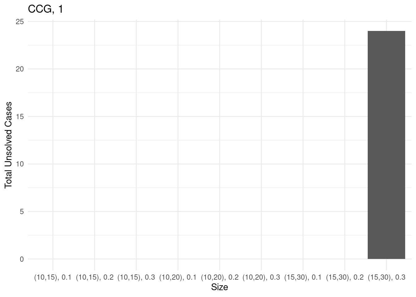
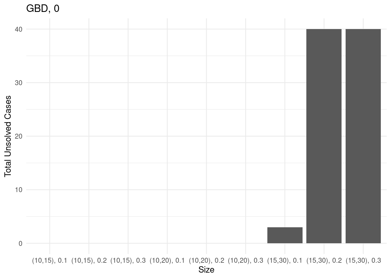
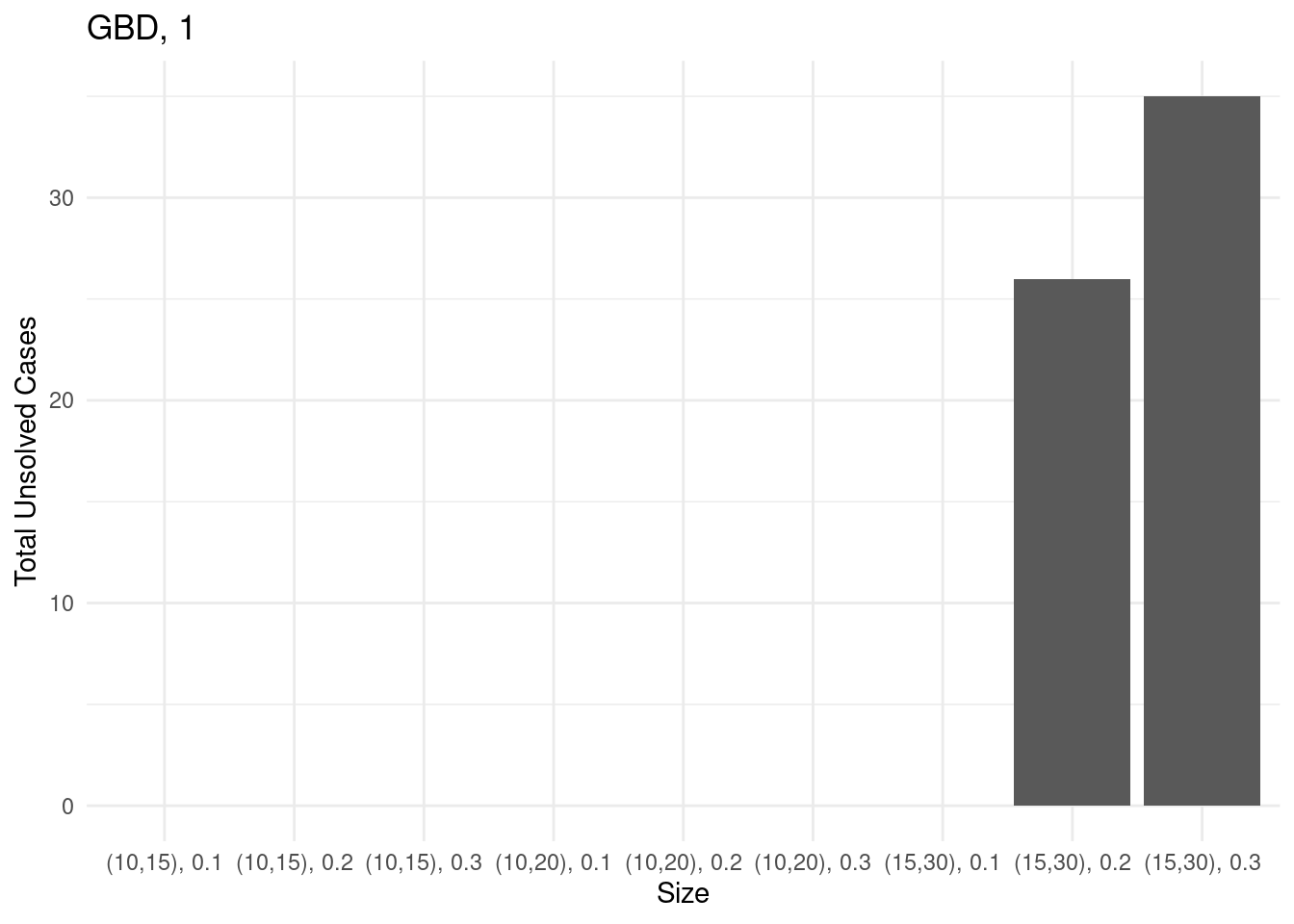
Unsolved instances
for (method in unique(results$method_extended)) {

  # Sum of unsolved cases for each size
  sum_unsolved = results[results$method_extended == method,] %>% group_by(size) %>% summarise(total_unsolved = sum(unsolved))

  # Create a bar plot
  p = ggplot(sum_unsolved, aes(x = size, y = total_unsolved)) +
    geom_bar(stat = "identity") +
    labs(x = "Size", y = "Total Unsolved Cases", title = method) +
    theme_minimal()

  ggsave(paste0("unsolved_", method, ".pdf"), plot = p, width = 10, height = 6)

  print(p)
}
Performance profiles and ECDF
We now introduce a function which plots the performance profile of our solvers over a given test set.
add_performance_ratio = function(dataset,
                                 criterion_column = "total_time",
                                 unsolved_column = "unsolved",
                                 instance_column = "instance",
                                 solver_column = "solver",
                                 output_column = "performance_ratio") {

  # Compute best score for each instance
  best = dataset %>%
    group_by(!!sym(instance_column)) %>%
    mutate(best_solver = min(!!sym(criterion_column)))

  # Compute performance ratio for each instance and solver
  result = best %>%
    group_by(!!sym(instance_column), !!sym(solver_column)) %>%
    mutate(!!sym(output_column) := !!sym(criterion_column) / best_solver) %>%
    ungroup()

  if (sum(result[,unsolved_column]) > 0) {
    result[result[,unsolved_column] == TRUE,output_column] = max(result[,output_column])
  }

  return (result)
}

plot_performance_profile = function(dataset,
                                    criterion_column,
                                    unsolved_column = "unsolved",
                                    instance_column = "instance",
                                    solver_column = "solver"
                                    ) {

  dataset_with_performance_ratios = add_performance_ratio(dataset,
                                                          criterion_column = criterion_column,
                                                          instance_column = instance_column,
                                                          solver_column = solver_column,
                                                          unsolved_column = unsolved_column)

  solved_dataset_with_performance_ratios = dataset_with_performance_ratios[!dataset_with_performance_ratios[,unsolved_column],]

  compute_performance_profile_point = function(method, data) {

    performance_ratios = solved_dataset_with_performance_ratios[solved_dataset_with_performance_ratios[,solver_column] == method,]$performance_ratio

    unscaled_performance_profile_point = ecdf(performance_ratios)(data)

    n_instances = sum(dataset[,solver_column] == method)
    n_solved_instances = sum(dataset[,solver_column] == method & !dataset[,unsolved_column])

    return( unscaled_performance_profile_point * n_solved_instances / n_instances )
  }

  perf = solved_dataset_with_performance_ratios %>%
    group_by(!!sym(solver_column)) %>%
    mutate(performance_profile_point = compute_performance_profile_point(unique(!!sym(solver_column)), performance_ratio))

  result = ggplot(data = perf, aes(x = performance_ratio, y = performance_profile_point, color = !!sym(solver_column))) +
              geom_line()

  return (result)
}
performance_profile = plot_performance_profile(results, criterion_column = "total_time", solver_column = "method_extended") +
labs(x = "Performance ratio", y = "% of instances") +
scale_y_continuous(limits = c(0, 1)) +
theme_minimal()
print(performance_profile)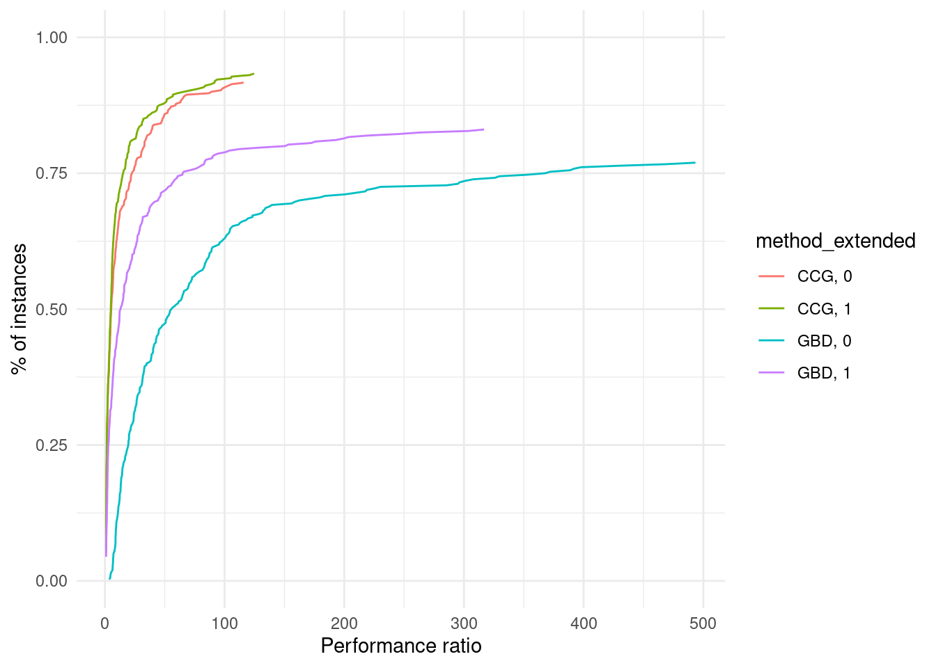
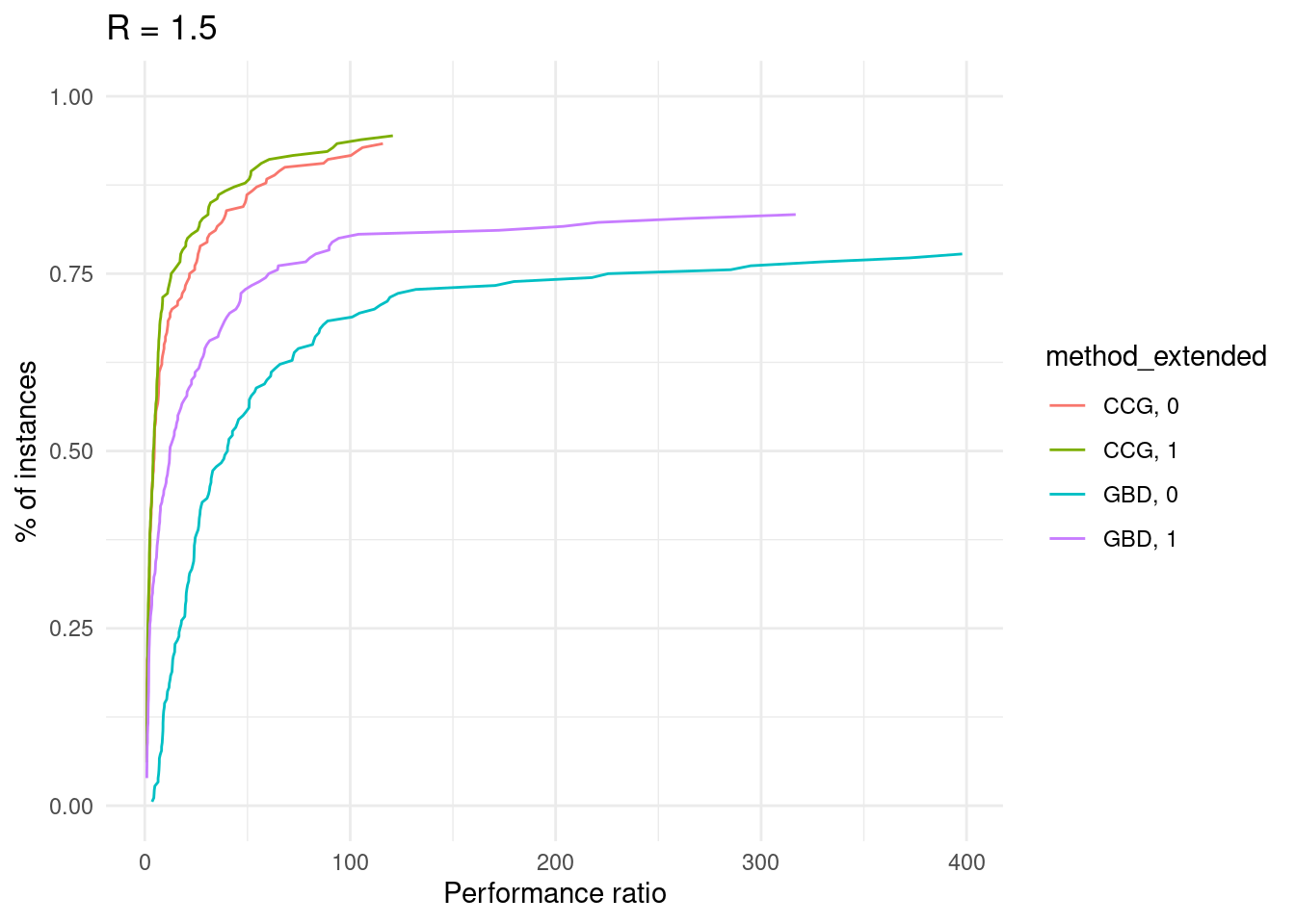
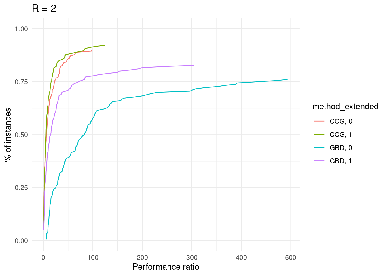
ggsave("performance_profile.pdf", plot = performance_profile)## Saving 7 x 5 in imagefor (ratio in unique(results$ratio_demand_capacity)) {
p = plot_performance_profile(results[results$ratio_demand_capacity == ratio,], criterion_column = "total_time", solver_column = "method_extended") +
labs(x = "Performance ratio", y = "% of instances", title = paste0("R = ", ratio / 1000)) +
scale_y_continuous(limits = c(0, 1)) +
theme_minimal()
print(p)
}
As a complement, we also draw the ECDF.
ggplot(results, aes(x = total_time, color = method_extended)) +
  stat_ecdf(geom = "step") +
  xlab("Total Time") +
  ylab("ECDF") +
  labs(title = "ECDF of Total Time by Method")  +
  scale_x_continuous(breaks = seq(0, max(results$total_time), by = 500), labels = seq(0, max(results$total_time), by = 500)) +
  theme_minimal()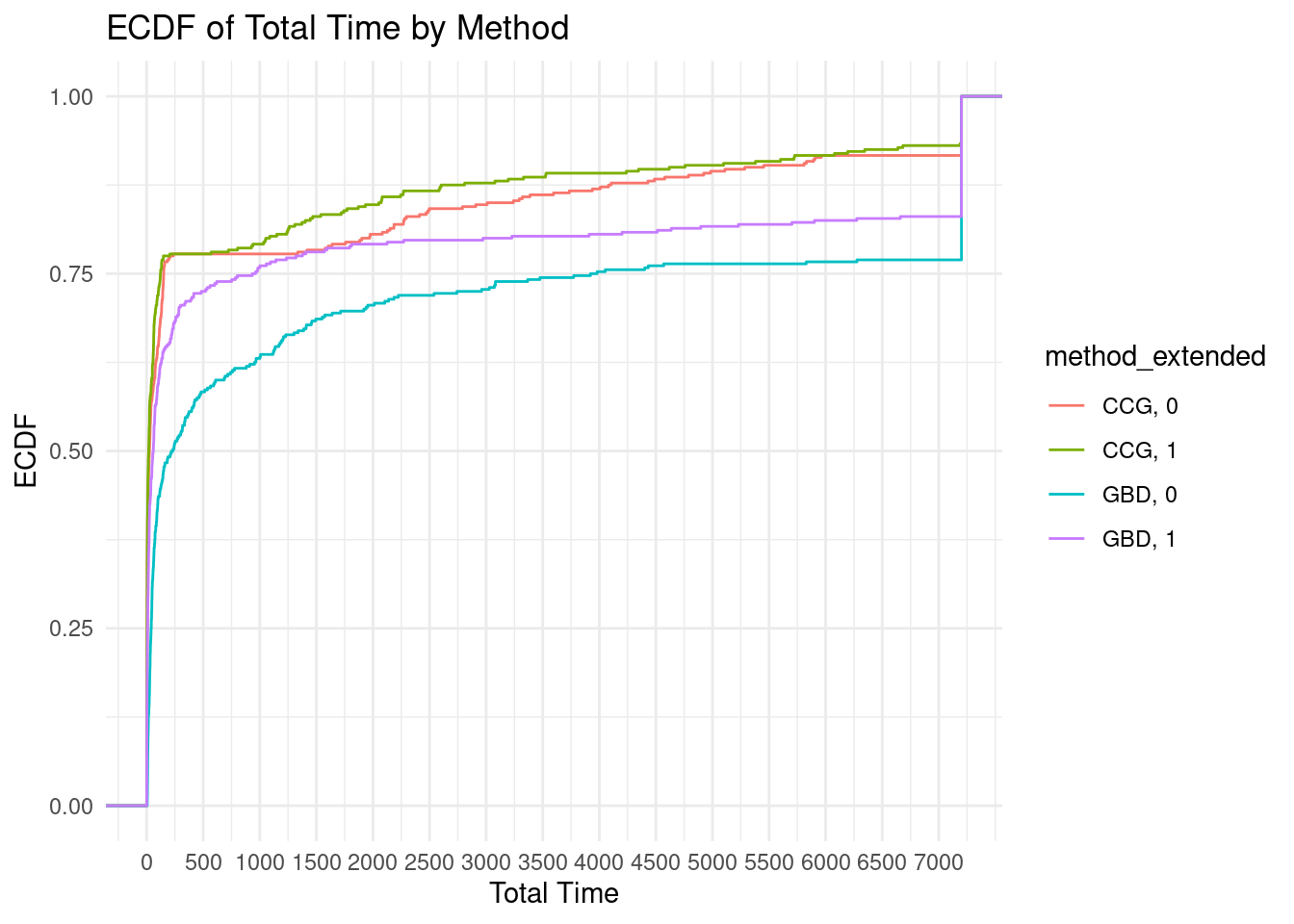
Summary table
In this section, we create a table summarizing the outcome of our experiments.
We start by computing average computation times over the solved instances.
results_solved = results %>%
  filter(total_time < 7200) %>%
  group_by(method_extended, n_facilities, n_customers, p, deviation) %>%
  summarize(
    solved = n(),
    total_time = mean(total_time),
    master_time = mean(master_time),
    separation_time = mean(separation_time),
    solved_iteration_count = mean(iteration_count),
    .groups = "drop"
  ) %>%
  ungroup()
Then, we also consider unsolved instances: we count the number of such instances and compute the average iteration count.
results_unsolved <- results %>%
  filter(total_time >= 7200) %>%
  group_by(method_extended, n_facilities, n_customers, p, deviation) %>%
  summarize(
    unsolved = n(),
    unsolved_iteration_count = mean(iteration_count),
    .groups = "drop"
  ) %>%
  ungroup()
We then merge the two tables.
final_result <- merge(results_solved, results_unsolved, by = c("method_extended", "n_facilities", "n_customers", "p", "deviation"), all = TRUE)Finally, we replace all NA entries by 0.
final_result[is.na(final_result)] = 0Here is our table.
|
Solved instances
|
Unsolved instances
|
||||||||||
|---|---|---|---|---|---|---|---|---|---|---|---|
| Method | |V_1| | |V_2| | p | dev | Count | Total | Master | Sepatation | # Iter | Count | # Iter |
| CCG, 0 | 10 | 15 | 0.1 | 0.25 | 20 | 1.25 | 0.52 | 0.68 | 2.25 | 0 | 0.00 |
| CCG, 0 | 10 | 15 | 0.1 | 0.50 | 20 | 1.22 | 0.50 | 0.67 | 2.20 | 0 | 0.00 |
| CCG, 0 | 10 | 15 | 0.2 | 0.25 | 20 | 3.94 | 0.55 | 3.34 | 2.25 | 0 | 0.00 |
| CCG, 0 | 10 | 15 | 0.2 | 0.50 | 20 | 4.76 | 0.64 | 4.06 | 2.45 | 0 | 0.00 |
| CCG, 0 | 10 | 15 | 0.3 | 0.25 | 20 | 7.91 | 0.86 | 6.99 | 2.75 | 0 | 0.00 |
| CCG, 0 | 10 | 15 | 0.3 | 0.50 | 20 | 7.71 | 0.69 | 6.96 | 2.65 | 0 | 0.00 |
| CCG, 0 | 10 | 20 | 0.1 | 0.25 | 20 | 4.98 | 0.94 | 3.98 | 2.50 | 0 | 0.00 |
| CCG, 0 | 10 | 20 | 0.1 | 0.50 | 20 | 5.03 | 0.94 | 4.03 | 2.55 | 0 | 0.00 |
| CCG, 0 | 10 | 20 | 0.2 | 0.25 | 20 | 26.35 | 1.01 | 25.29 | 2.65 | 0 | 0.00 |
| CCG, 0 | 10 | 20 | 0.2 | 0.50 | 20 | 26.58 | 0.97 | 25.54 | 2.70 | 0 | 0.00 |
| CCG, 0 | 10 | 20 | 0.3 | 0.25 | 20 | 83.87 | 0.95 | 82.85 | 2.70 | 0 | 0.00 |
| CCG, 0 | 10 | 20 | 0.3 | 0.50 | 20 | 88.27 | 0.83 | 87.38 | 2.70 | 0 | 0.00 |
| CCG, 0 | 15 | 30 | 0.1 | 0.25 | 20 | 129.85 | 4.12 | 125.60 | 2.90 | 0 | 0.00 |
| CCG, 0 | 15 | 30 | 0.1 | 0.50 | 20 | 131.51 | 4.23 | 127.16 | 2.95 | 0 | 0.00 |
| CCG, 0 | 15 | 30 | 0.2 | 0.25 | 20 | 2969.99 | 4.79 | 2965.07 | 3.10 | 0 | 0.00 |
| CCG, 0 | 15 | 30 | 0.2 | 0.50 | 20 | 3027.15 | 4.61 | 3022.41 | 3.10 | 0 | 0.00 |
| CCG, 0 | 15 | 30 | 0.3 | 0.25 | 5 | 4303.16 | 2.27 | 4300.79 | 2.60 | 15 | 1.40 |
| CCG, 0 | 15 | 30 | 0.3 | 0.50 | 5 | 4833.15 | 2.15 | 4830.88 | 2.60 | 15 | 1.40 |
| CCG, 1 | 10 | 15 | 0.1 | 0.25 | 20 | 1.99 | 1.47 | 0.46 | 3.40 | 0 | 0.00 |
| CCG, 1 | 10 | 15 | 0.1 | 0.50 | 20 | 1.97 | 1.43 | 0.48 | 3.40 | 0 | 0.00 |
| CCG, 1 | 10 | 15 | 0.2 | 0.25 | 20 | 4.08 | 1.63 | 2.37 | 3.75 | 0 | 0.00 |
| CCG, 1 | 10 | 15 | 0.2 | 0.50 | 20 | 5.01 | 1.62 | 3.31 | 3.85 | 0 | 0.00 |
| CCG, 1 | 10 | 15 | 0.3 | 0.25 | 20 | 6.35 | 1.99 | 4.28 | 4.10 | 0 | 0.00 |
| CCG, 1 | 10 | 15 | 0.3 | 0.50 | 20 | 6.83 | 1.69 | 5.06 | 4.05 | 0 | 0.00 |
| CCG, 1 | 10 | 20 | 0.1 | 0.25 | 20 | 4.81 | 2.20 | 2.53 | 3.65 | 0 | 0.00 |
| CCG, 1 | 10 | 20 | 0.1 | 0.50 | 20 | 4.94 | 2.20 | 2.66 | 3.70 | 0 | 0.00 |
| CCG, 1 | 10 | 20 | 0.2 | 0.25 | 20 | 19.99 | 2.45 | 17.45 | 3.95 | 0 | 0.00 |
| CCG, 1 | 10 | 20 | 0.2 | 0.50 | 20 | 20.05 | 2.17 | 17.79 | 3.90 | 0 | 0.00 |
| CCG, 1 | 10 | 20 | 0.3 | 0.25 | 20 | 56.29 | 2.87 | 53.34 | 4.30 | 0 | 0.00 |
| CCG, 1 | 10 | 20 | 0.3 | 0.50 | 20 | 71.35 | 2.37 | 68.90 | 4.10 | 0 | 0.00 |
| CCG, 1 | 15 | 30 | 0.1 | 0.25 | 20 | 85.53 | 8.72 | 76.65 | 3.95 | 0 | 0.00 |
| CCG, 1 | 15 | 30 | 0.1 | 0.50 | 20 | 82.50 | 7.78 | 74.57 | 3.80 | 0 | 0.00 |
| CCG, 1 | 15 | 30 | 0.2 | 0.25 | 20 | 1730.38 | 11.12 | 1719.08 | 4.55 | 0 | 0.00 |
| CCG, 1 | 15 | 30 | 0.2 | 0.50 | 20 | 2359.21 | 11.34 | 2347.68 | 4.50 | 0 | 0.00 |
| CCG, 1 | 15 | 30 | 0.3 | 0.25 | 10 | 5406.71 | 10.22 | 5396.31 | 4.50 | 10 | 3.70 |
| CCG, 1 | 15 | 30 | 0.3 | 0.50 | 6 | 3827.73 | 9.50 | 3818.05 | 4.50 | 14 | 3.00 |
| GBD, 0 | 10 | 15 | 0.1 | 0.25 | 20 | 9.63 | 0.59 | 9.00 | 31.95 | 0 | 0.00 |
| GBD, 0 | 10 | 15 | 0.1 | 0.50 | 20 | 9.41 | 0.56 | 8.81 | 31.15 | 0 | 0.00 |
| GBD, 0 | 10 | 15 | 0.2 | 0.25 | 20 | 43.64 | 0.55 | 43.04 | 29.95 | 0 | 0.00 |
| GBD, 0 | 10 | 15 | 0.2 | 0.50 | 20 | 43.41 | 0.47 | 42.89 | 27.55 | 0 | 0.00 |
| GBD, 0 | 10 | 15 | 0.3 | 0.25 | 20 | 71.43 | 0.52 | 70.86 | 29.65 | 0 | 0.00 |
| GBD, 0 | 10 | 15 | 0.3 | 0.50 | 20 | 63.00 | 0.44 | 62.52 | 25.15 | 0 | 0.00 |
| GBD, 0 | 10 | 20 | 0.1 | 0.25 | 20 | 48.39 | 0.66 | 47.67 | 31.90 | 0 | 0.00 |
| GBD, 0 | 10 | 20 | 0.1 | 0.50 | 20 | 47.93 | 0.64 | 47.24 | 30.95 | 0 | 0.00 |
| GBD, 0 | 10 | 20 | 0.2 | 0.25 | 20 | 294.82 | 0.65 | 294.12 | 31.35 | 0 | 0.00 |
| GBD, 0 | 10 | 20 | 0.2 | 0.50 | 20 | 277.99 | 0.61 | 277.33 | 29.15 | 0 | 0.00 |
| GBD, 0 | 10 | 20 | 0.3 | 0.25 | 20 | 894.53 | 0.56 | 893.92 | 29.45 | 0 | 0.00 |
| GBD, 0 | 10 | 20 | 0.3 | 0.50 | 20 | 856.88 | 0.57 | 856.26 | 27.85 | 0 | 0.00 |
| GBD, 0 | 15 | 30 | 0.1 | 0.25 | 18 | 2401.50 | 4.62 | 2396.76 | 66.17 | 2 | 170.00 |
| GBD, 0 | 15 | 30 | 0.1 | 0.50 | 19 | 2765.66 | 5.43 | 2760.10 | 71.95 | 1 | 207.00 |
| GBD, 0 | 15 | 30 | 0.2 | 0.25 | 0 | 0.00 | 0.00 | 0.00 | 0.00 | 20 | 9.65 |
| GBD, 0 | 15 | 30 | 0.2 | 0.50 | 0 | 0.00 | 0.00 | 0.00 | 0.00 | 20 | 9.80 |
| GBD, 0 | 15 | 30 | 0.3 | 0.25 | 0 | 0.00 | 0.00 | 0.00 | 0.00 | 20 | 2.85 |
| GBD, 0 | 15 | 30 | 0.3 | 0.50 | 0 | 0.00 | 0.00 | 0.00 | 0.00 | 20 | 2.65 |
| GBD, 1 | 10 | 15 | 0.1 | 0.25 | 20 | 2.25 | 0.70 | 1.49 | 34.30 | 0 | 0.00 |
| GBD, 1 | 10 | 15 | 0.1 | 0.50 | 20 | 4.12 | 0.67 | 3.40 | 34.00 | 0 | 0.00 |
| GBD, 1 | 10 | 15 | 0.2 | 0.25 | 20 | 9.30 | 0.69 | 8.55 | 33.45 | 0 | 0.00 |
| GBD, 1 | 10 | 15 | 0.2 | 0.50 | 20 | 16.39 | 0.58 | 15.76 | 30.75 | 0 | 0.00 |
| GBD, 1 | 10 | 15 | 0.3 | 0.25 | 20 | 31.25 | 0.69 | 30.51 | 33.85 | 0 | 0.00 |
| GBD, 1 | 10 | 15 | 0.3 | 0.50 | 20 | 28.69 | 0.55 | 28.09 | 28.95 | 0 | 0.00 |
| GBD, 1 | 10 | 20 | 0.1 | 0.25 | 20 | 12.60 | 0.77 | 11.77 | 35.15 | 0 | 0.00 |
| GBD, 1 | 10 | 20 | 0.1 | 0.50 | 20 | 10.50 | 0.73 | 9.72 | 34.30 | 0 | 0.00 |
| GBD, 1 | 10 | 20 | 0.2 | 0.25 | 20 | 101.11 | 0.86 | 100.21 | 36.75 | 0 | 0.00 |
| GBD, 1 | 10 | 20 | 0.2 | 0.50 | 20 | 114.80 | 0.69 | 114.07 | 32.10 | 0 | 0.00 |
| GBD, 1 | 10 | 20 | 0.3 | 0.25 | 20 | 252.38 | 0.78 | 251.54 | 34.35 | 0 | 0.00 |
| GBD, 1 | 10 | 20 | 0.3 | 0.50 | 20 | 367.06 | 0.73 | 366.28 | 32.55 | 0 | 0.00 |
| GBD, 1 | 15 | 30 | 0.1 | 0.25 | 20 | 344.79 | 8.99 | 335.66 | 83.30 | 0 | 0.00 |
| GBD, 1 | 15 | 30 | 0.1 | 0.50 | 20 | 624.76 | 9.10 | 615.52 | 87.55 | 0 | 0.00 |
| GBD, 1 | 15 | 30 | 0.2 | 0.25 | 9 | 2678.95 | 11.49 | 2667.30 | 91.11 | 11 | 40.27 |
| GBD, 1 | 15 | 30 | 0.2 | 0.50 | 5 | 3185.92 | 6.81 | 3178.95 | 85.80 | 15 | 59.87 |
| GBD, 1 | 15 | 30 | 0.3 | 0.25 | 3 | 5379.95 | 7.06 | 5372.76 | 77.67 | 17 | 85.35 |
| GBD, 1 | 15 | 30 | 0.3 | 0.50 | 2 | 4402.85 | 5.80 | 4396.92 | 75.00 | 18 | 60.94 |
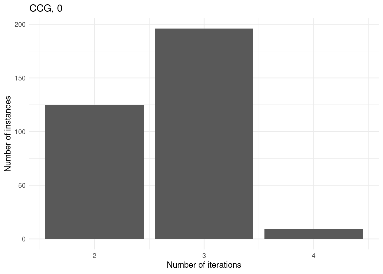
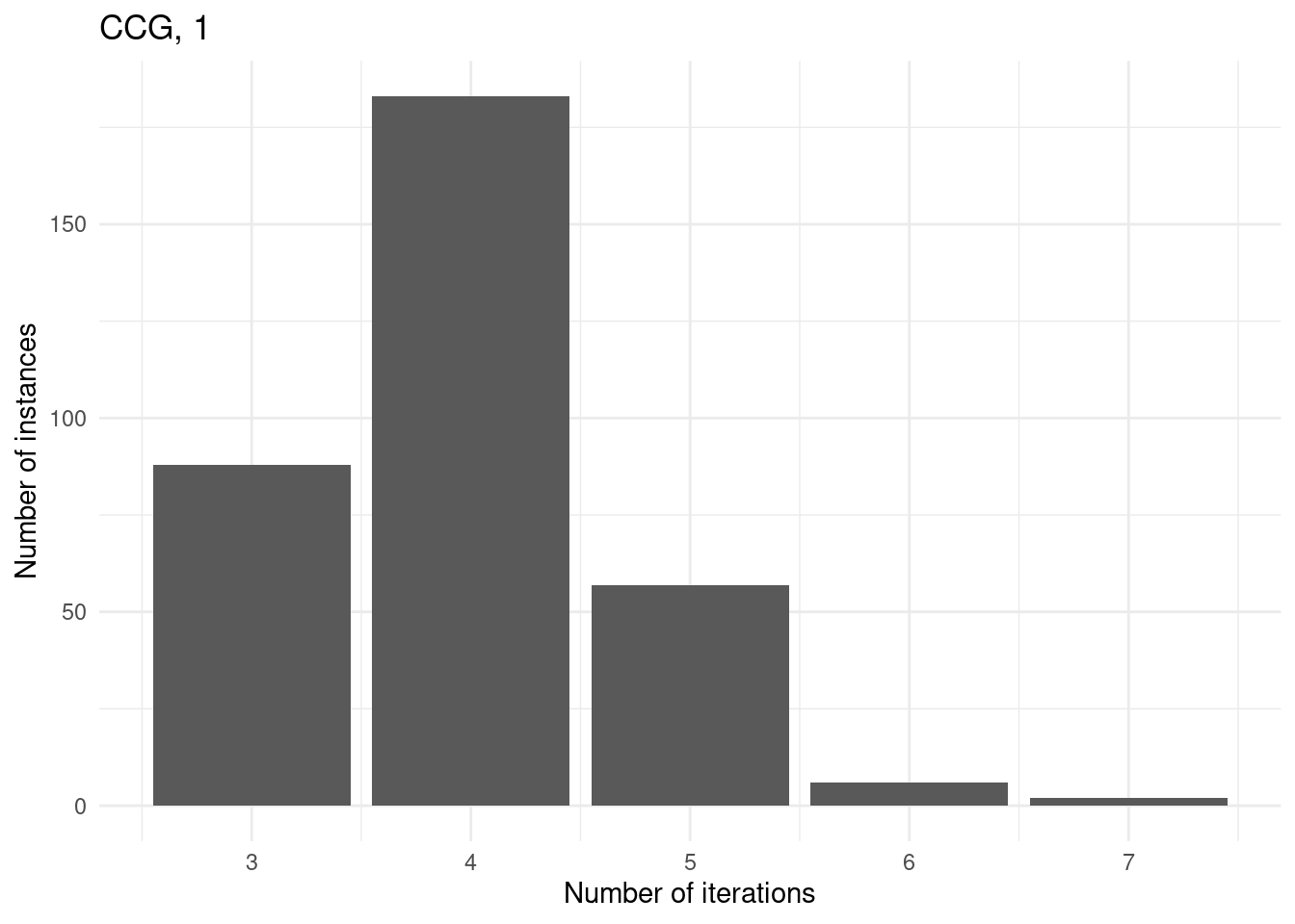
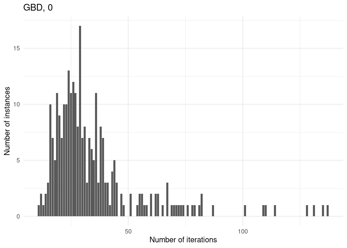
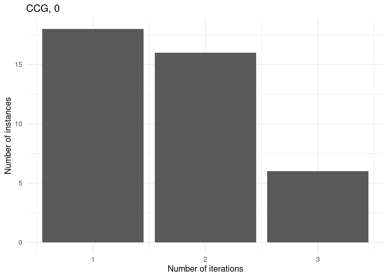
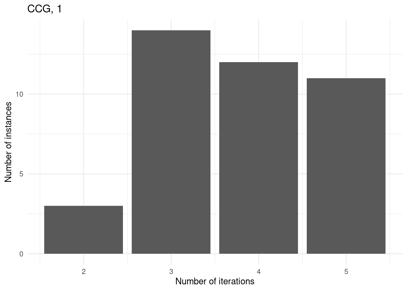
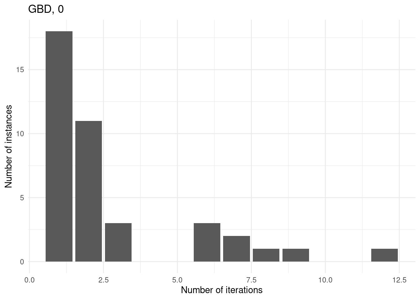
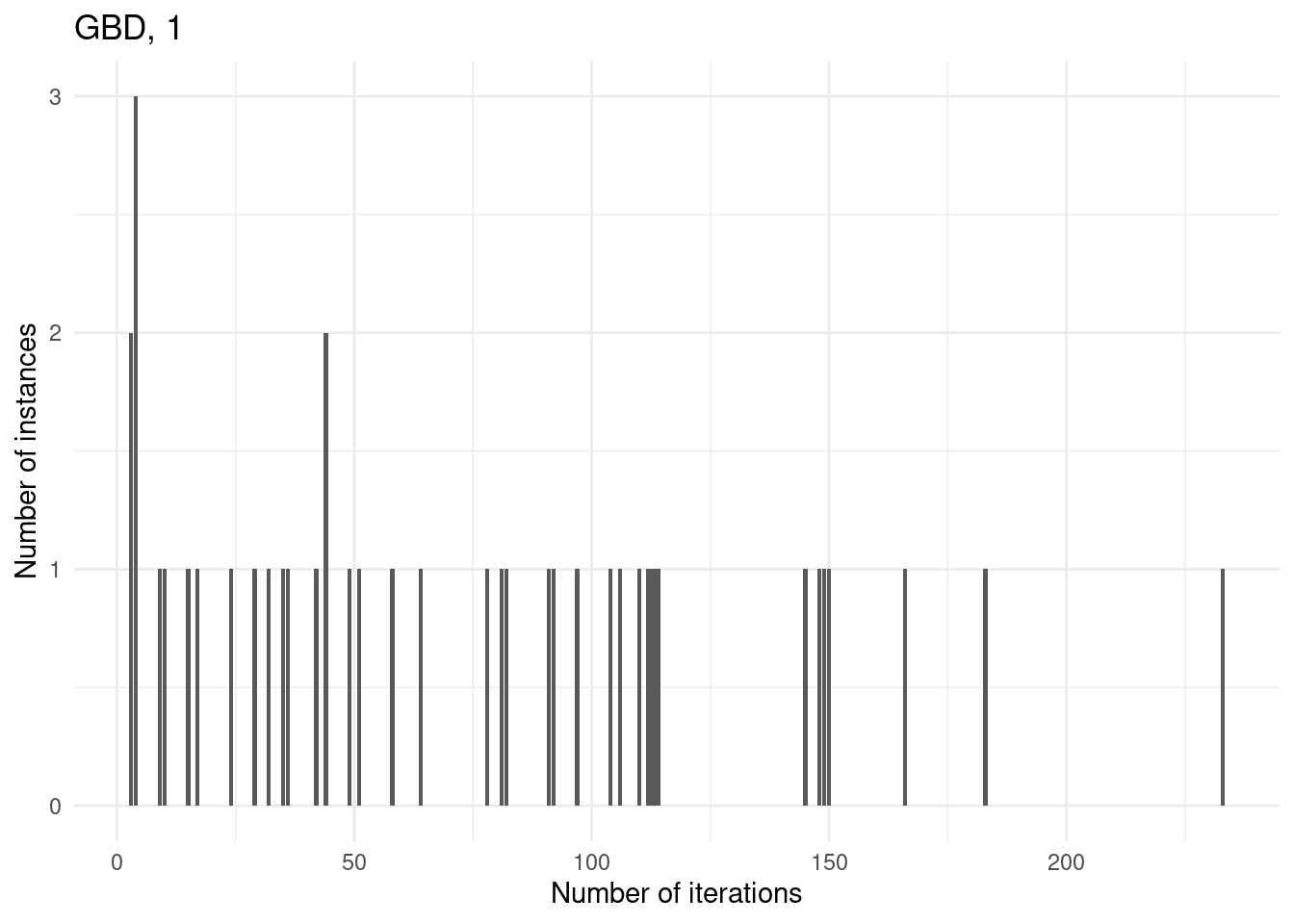
Number of iterations
for (method in unique(results$method_extended)) {

  p = ggplot(results[results$method_extended == method & results$total_time < time_limit,], aes(x = iteration_count)) +
    geom_bar() +
    labs(
      title = method,
      x = "Number of iterations",
      y = "Number of instances"
    ) +
    theme_minimal()

  print(p)
}
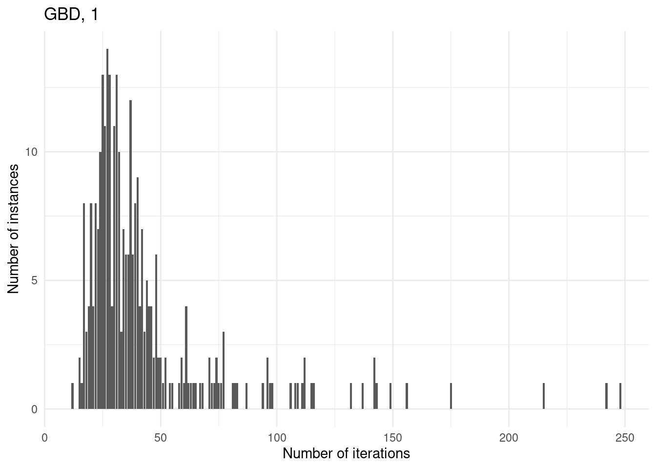
Understanding unsolved instances
We first consider those instances with 15 facilities and p = 0.3 since these are the instances which both approaches cannot solve at all.
subset = results[results$n_facilities == 15 & results$p > .25,]Then, observe how, for the subset of instances such that iteration_count is 1 for at least one of the methods, the computation times are the same (which makes sense because, actually, the same routines are executed - intial master and first separation).
filtered_subset = subset %>%
  group_by(instance) %>%
  filter(any(iteration_count < 1))

ggplot(filtered_subset, aes(x = method, y = master_time)) +
  geom_boxplot() +
  labs(x = "Method", y = "Master time") +
  theme_minimal()
ggplot(filtered_subset, aes(x = method, y = separation_time)) +
  geom_boxplot() +
  labs(x = "Method", y = "Separation time") +
  theme_minimal()
However, for some instances, GBD can do more iterations because the master problem is nicer whereas CCG has a convex MINLP problem which he cannot solve within the time limit.
for (method in unique(subset$method_extended)) {

  p = ggplot(subset[subset$method_extended == method,], aes(x = iteration_count)) +
    geom_bar() +
    labs(
      title = method,
      x = "Number of iterations",
      y = "Number of instances"
    ) +
    theme_minimal()

  print(p)
}
This document is automatically generated after every
git push action on the public repository
hlefebvr/hlefebvr.github.io using rmarkdown and Github
Actions. This ensures the reproducibility of our data manipulation. The
last compilation was performed on the 12/09/24 14:05:36.