Table of content
Open methodology for “Exact approach for convex adjustable robust optimization > Resource Allocation Problem (RAP)
Loading the data
The raw results can be found in the file results.csv
with the following columns:
- tag: a tag which should always equal “result” used to
grepthe result line in the execution log file. - instance: the name or path of the instance.
- n_servers: the number of servers in the instance.
- n_clients: the number of clients in the instance.
- Gamma: the value of \(\Gamma\) which was used.
- deviation: the maximum deviation, in percentage, from the nominal demand.
- time_limit: the time limit which was used when solving the instance.
- method: the name of the method which was used to solve the instance.
- total_time: the total time used to solve the instance.
- master_time: the time spent solving the master problem.
- separation_time: the time spent solving the separation problem.
- best_bound: the best bound found.
- iteration_count: the number of iterations.
- fail: should be empty if the execution of the algorithm went well.
We start by reading the file and by removing the “tag” column.
results = read.table("./new-results.csv", header = FALSE, sep = ',')
colnames(results) <- c("tag", "instance", "n_servers", "n_clients", "Gamma", "deviation", "time_limit", "method", "use_heuristic", "total_time", "master_time", "separation_time", "best_bound", "iteration_count", "fail")
results$tag = NULL
Then, we compute the percentage which \(\Gamma\) represents for the total number of clients.
results$p = results$Gamma / results$n_clients
results$p = ceiling(results$p / .05) * .05
results$size = paste0("(", results$n_servers, ",", results$n_clients, "), ", results$p)results$method_extended = paste0(results$method, ", ", results$use_heuristic)We also get rid of instances which were too large to be solved by both approaches.
results = results[!(results$n_clients == 40),]
results = results[!(results$n_servers == 25 & results$n_clients == 25),]
We then check that all instances were solved without issue by checking the “fail” column.
sum(results$fail)## [1] 62We add a tag for unsolved instances.
time_limit = 7200

if (sum(results$fail) > 0) {
  results[results$fail == TRUE,]$total_time = time_limit
}

results$unsolved = results$total_time >= time_limit | results$fail
All in all, our result data reads.
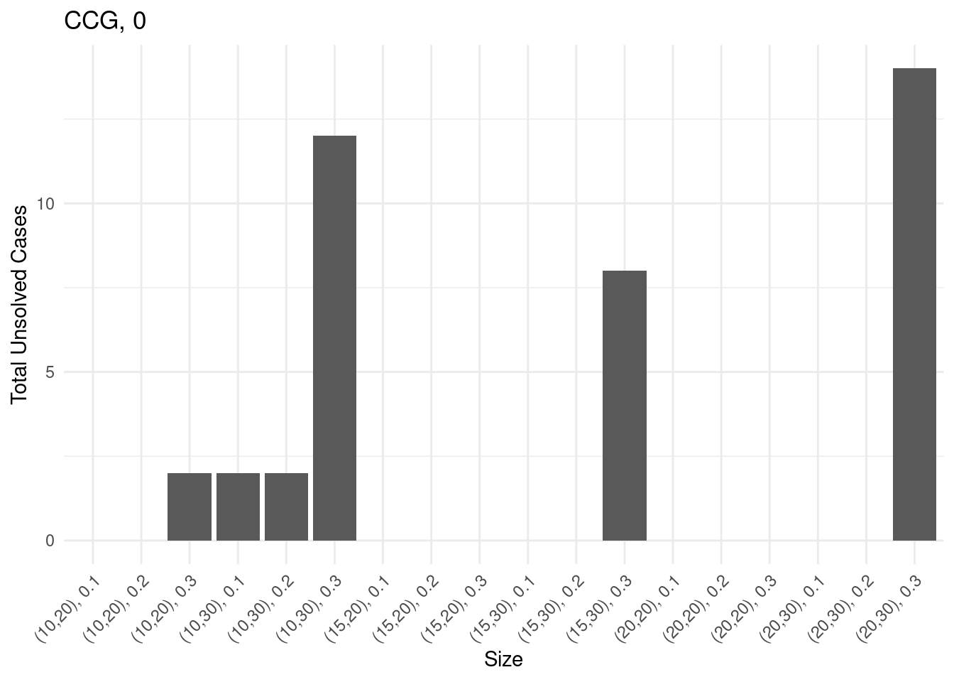
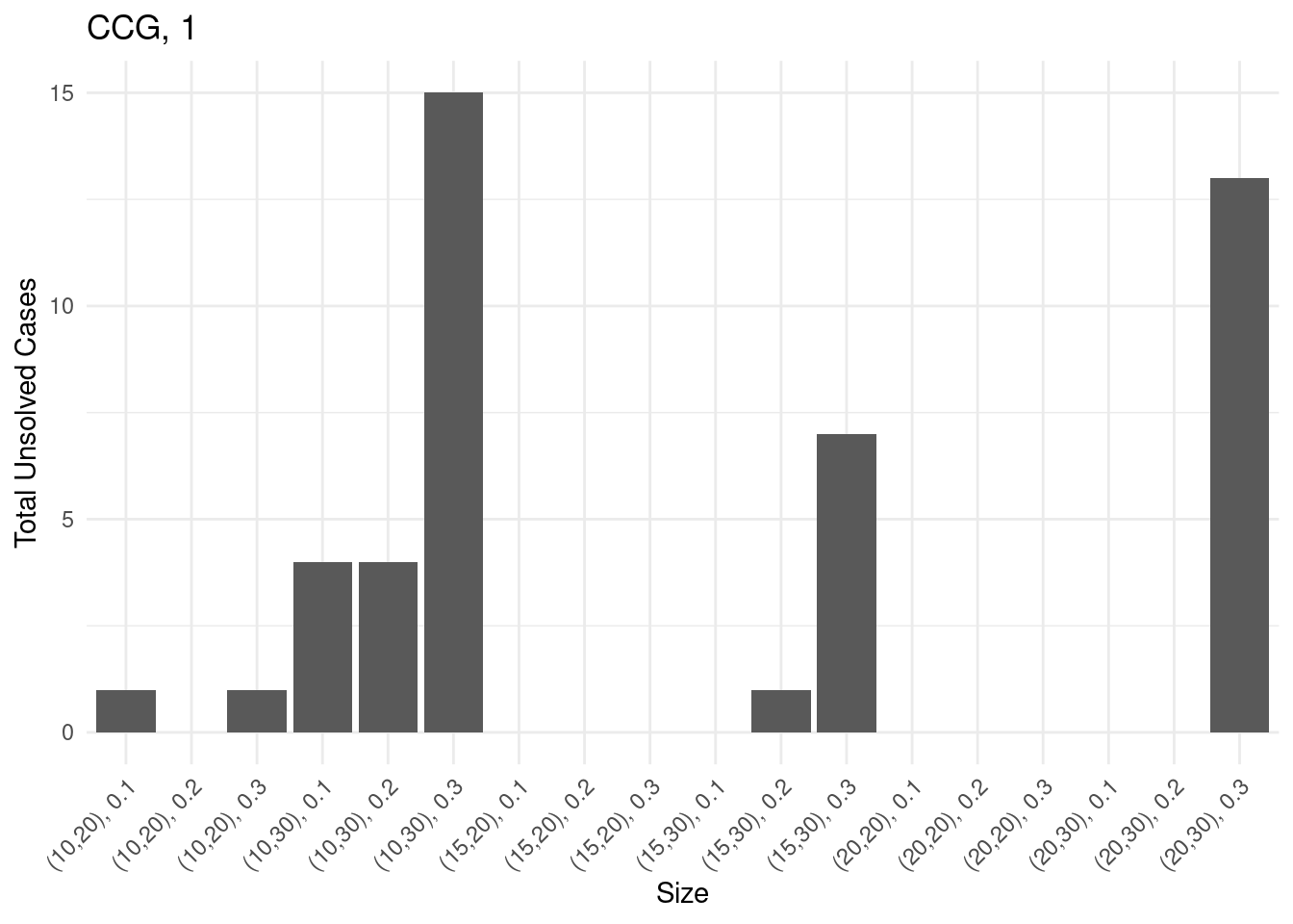
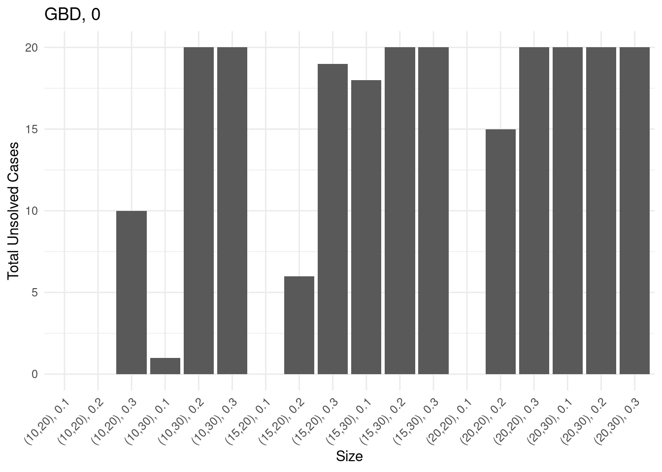
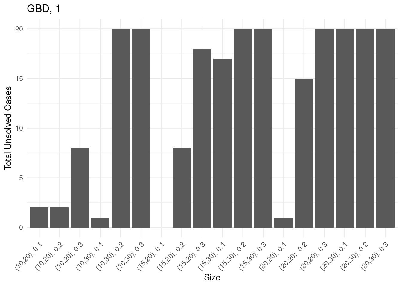
Unsolved instances
for (method in unique(results$method_extended)) {

  # Sum of unsolved cases for each size
  sum_unsolved = results[results$method_extended == method,] %>% group_by(size) %>% summarise(total_unsolved = sum(unsolved))

  # Create a bar plot
  p = ggplot(sum_unsolved, aes(x = size, y = total_unsolved)) +
    geom_bar(stat = "identity") +
    labs(x = "Size", y = "Total Unsolved Cases", title = method) +
    theme_minimal() +
    theme(axis.text.x = element_text(angle = 45, hjust = 1))

  ggsave(paste0("unsolved_", method, ".pdf"), plot = p, width = 10, height = 6)

  print(p)
}
Performance profiles and ECDF
We now introduce a function which plots the performance profile of our solvers over a given test set.
add_performance_ratio = function(dataset,
                                 criterion_column = "total_time",
                                 unsolved_column = "unsolved",
                                 instance_column = "instance",
                                 solver_column = "solver",
                                 output_column = "performance_ratio") {

  # Compute best score for each instance
  best = dataset %>%
    group_by(!!sym(instance_column)) %>%
    mutate(best_solver = min(!!sym(criterion_column)))

  # Compute performance ratio for each instance and solver
  result = best %>%
    group_by(!!sym(instance_column), !!sym(solver_column)) %>%
    mutate(!!sym(output_column) := !!sym(criterion_column) / best_solver) %>%
    ungroup()

  if (sum(result[,unsolved_column]) > 0) {
    result[result[,unsolved_column] == TRUE,output_column] = max(result[,output_column])
  }

  return (result)
}

plot_performance_profile = function(dataset,
                                    criterion_column,
                                    unsolved_column = "unsolved",
                                    instance_column = "instance",
                                    solver_column = "solver"
                                    ) {

  dataset_with_performance_ratios = add_performance_ratio(dataset,
                                                          criterion_column = criterion_column,
                                                          instance_column = instance_column,
                                                          solver_column = solver_column,
                                                          unsolved_column = unsolved_column)

  solved_dataset_with_performance_ratios = dataset_with_performance_ratios[!dataset_with_performance_ratios[,unsolved_column],]

  compute_performance_profile_point = function(method, data) {

    performance_ratios = solved_dataset_with_performance_ratios[solved_dataset_with_performance_ratios[,solver_column] == method,]$performance_ratio

    unscaled_performance_profile_point = ecdf(performance_ratios)(data)

    n_instances = sum(dataset[,solver_column] == method)
    n_solved_instances = sum(dataset[,solver_column] == method & !dataset[,unsolved_column])

    return( unscaled_performance_profile_point * n_solved_instances / n_instances )
  }

  perf = solved_dataset_with_performance_ratios %>%
    group_by(!!sym(solver_column)) %>%
    mutate(performance_profile_point = compute_performance_profile_point(unique(!!sym(solver_column)), performance_ratio))

  result = ggplot(data = perf, aes(x = performance_ratio, y = performance_profile_point, color = !!sym(solver_column))) +
              geom_line()

  return (result)
}
performance_profile = plot_performance_profile(results, criterion_column = "total_time", solver_column = "method_extended") +
labs(x = "Performance ratio", y = "% of instances") +
scale_y_continuous(limits = c(0, 1)) +
theme_minimal()
print(performance_profile)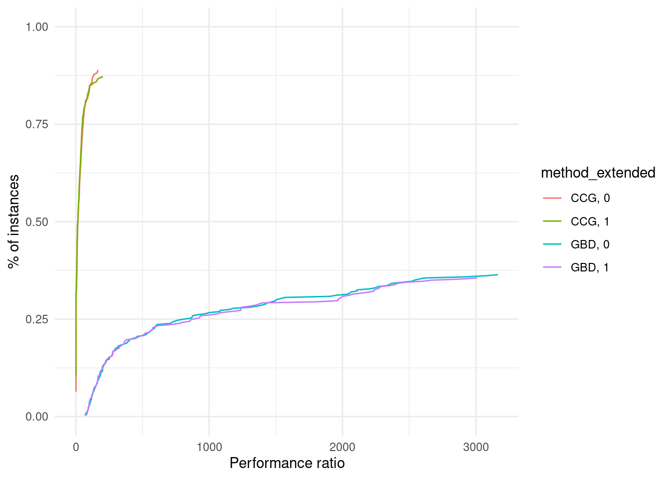
ggsave("performance_profile.pdf", plot = performance_profile)## Saving 7 x 5 in imageAs a complement, we also draw the ECDF.
ggplot(results, aes(x = total_time, color = method_extended)) +
  stat_ecdf(geom = "step") +
  xlab("Total Time") +
  ylab("ECDF") +
  labs(title = "ECDF of Total Time by Method")  +
  scale_x_continuous(breaks = seq(0, max(results$total_time), by = 500), labels = seq(0, max(results$total_time), by = 500)) +
  theme_minimal()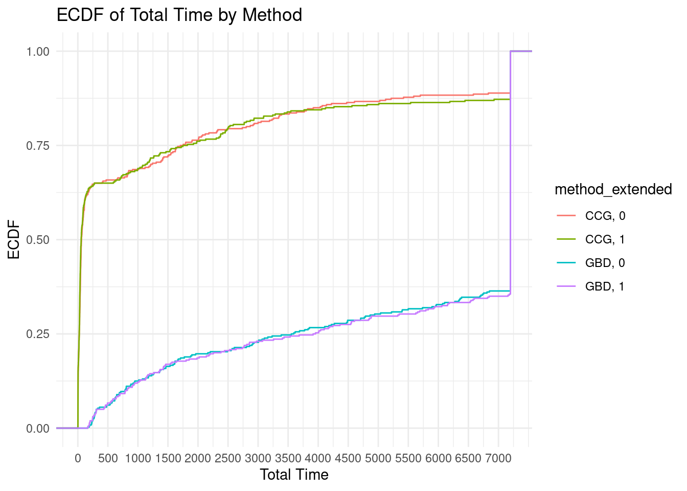
Summary table
In this section, we create a table summarizing the outcome of our experiments.
We start by computing average computation times over the solved instances.
results_solved = results %>%
  filter(total_time < time_limit) %>%
  group_by(method_extended, n_servers, n_clients, p, deviation) %>%
  summarize(
    solved = n(),
    total_time = mean(total_time),
    master_time = mean(master_time),
    separation_time = mean(separation_time),
    solved_iteration_count = mean(iteration_count),
    .groups = "drop"
  ) %>%
  ungroup()
Then, we also consider unsolved instances: we count the number of such instances and compute the average iteration count.
results_unsolved <- results %>%
  filter(total_time >= time_limit) %>%
  group_by(method_extended, n_servers, n_clients, p, deviation) %>%
  summarize(
    unsolved = n(),
    unsolved_iteration_count = mean(iteration_count),
    .groups = "drop"
  ) %>%
  ungroup()

results_fail <- results %>%
  filter(fail == TRUE) %>%
  group_by(method_extended, n_servers, n_clients, p, deviation) %>%
  summarize(
    fail = n(),
    .groups = "drop"
  ) %>%
  ungroup()
We then merge the two tables.
final_result <- merge(results_solved, results_unsolved, by = c("method_extended", "n_servers", "n_clients", "p", "deviation"), all = TRUE)
final_result <- merge(final_result, results_fail, by = c("method_extended", "n_servers", "n_clients", "p", "deviation"), all = TRUE)
Here is our table.
|
Solved instances
|
Unsolved instances
|
|||||||||||
|---|---|---|---|---|---|---|---|---|---|---|---|---|
| Method | |V_1| | |V_2| | p | dev | Count | Total | Master | Sepatation | # Iter | Count | # Iter | # Errors |
| CCG, 0 | 10 | 20 | 0.1 | 0.25 | 10 | 2.76 | 0.07 | 2.64 | 2.80 | NA | NA | NA |
| CCG, 0 | 10 | 20 | 0.1 | 0.50 | 10 | 2.79 | 0.06 | 2.67 | 3.00 | NA | NA | NA |
| CCG, 0 | 10 | 20 | 0.2 | 0.25 | 10 | 20.97 | 0.06 | 20.85 | 3.00 | NA | NA | NA |
| CCG, 0 | 10 | 20 | 0.2 | 0.50 | 10 | 18.75 | 0.06 | 18.63 | 2.80 | NA | NA | NA |
| CCG, 0 | 10 | 20 | 0.3 | 0.25 | 10 | 64.48 | 0.08 | 64.32 | 3.00 | NA | NA | NA |
| CCG, 0 | 10 | 20 | 0.3 | 0.50 | 8 | 67.37 | 0.05 | 67.27 | 2.88 | 2 | 28.00 | 2 |
| CCG, 0 | 10 | 30 | 0.1 | 0.25 | 8 | 41.15 | 0.07 | 41.00 | 2.62 | 2 | 2.50 | 2 |
| CCG, 0 | 10 | 30 | 0.1 | 0.50 | 10 | 51.68 | 0.09 | 51.50 | 3.00 | NA | NA | NA |
| CCG, 0 | 10 | 30 | 0.2 | 0.25 | 9 | 1679.41 | 0.09 | 1679.23 | 3.11 | 1 | 1.00 | 1 |
| CCG, 0 | 10 | 30 | 0.2 | 0.50 | 9 | 1686.99 | 0.09 | 1686.81 | 3.11 | 1 | 2.00 | 1 |
| CCG, 0 | 10 | 30 | 0.3 | 0.25 | 4 | 3209.94 | 0.07 | 3209.79 | 2.50 | 6 | 1.83 | 2 |
| CCG, 0 | 10 | 30 | 0.3 | 0.50 | 4 | 3085.95 | 0.07 | 3085.81 | 2.50 | 6 | 1.67 | 1 |
| CCG, 0 | 15 | 20 | 0.1 | 0.25 | 10 | 3.60 | 0.08 | 3.44 | 2.80 | NA | NA | NA |
| CCG, 0 | 15 | 20 | 0.1 | 0.50 | 10 | 3.49 | 0.10 | 3.32 | 2.60 | NA | NA | NA |
| CCG, 0 | 15 | 20 | 0.2 | 0.25 | 10 | 30.09 | 0.09 | 29.91 | 2.80 | NA | NA | NA |
| CCG, 0 | 15 | 20 | 0.2 | 0.50 | 10 | 30.52 | 0.07 | 30.38 | 2.70 | NA | NA | NA |
| CCG, 0 | 15 | 20 | 0.3 | 0.25 | 10 | 138.92 | 0.11 | 138.73 | 3.00 | NA | NA | NA |
| CCG, 0 | 15 | 20 | 0.3 | 0.50 | 10 | 131.24 | 0.08 | 131.08 | 2.90 | NA | NA | NA |
| CCG, 0 | 15 | 30 | 0.1 | 0.25 | 10 | 50.36 | 0.13 | 50.11 | 3.00 | NA | NA | NA |
| CCG, 0 | 15 | 30 | 0.1 | 0.50 | 10 | 54.69 | 0.13 | 54.44 | 3.20 | NA | NA | NA |
| CCG, 0 | 15 | 30 | 0.2 | 0.25 | 10 | 1945.35 | 0.14 | 1945.08 | 3.50 | NA | NA | NA |
| CCG, 0 | 15 | 30 | 0.2 | 0.50 | 10 | 1916.98 | 0.13 | 1916.73 | 3.40 | NA | NA | NA |
| CCG, 0 | 15 | 30 | 0.3 | 0.25 | 6 | 4018.79 | 0.10 | 4018.58 | 3.17 | 4 | 1.50 | NA |
| CCG, 0 | 15 | 30 | 0.3 | 0.50 | 6 | 3568.58 | 0.11 | 3568.36 | 3.00 | 4 | 1.75 | NA |
| CCG, 0 | 20 | 20 | 0.1 | 0.25 | 10 | 4.34 | 0.11 | 4.14 | 2.80 | NA | NA | NA |
| CCG, 0 | 20 | 20 | 0.1 | 0.50 | 10 | 4.71 | 0.11 | 4.50 | 2.90 | NA | NA | NA |
| CCG, 0 | 20 | 20 | 0.2 | 0.25 | 10 | 37.34 | 0.10 | 37.14 | 2.90 | NA | NA | NA |
| CCG, 0 | 20 | 20 | 0.2 | 0.50 | 10 | 40.38 | 0.12 | 40.16 | 3.20 | NA | NA | NA |
| CCG, 0 | 20 | 20 | 0.3 | 0.25 | 10 | 120.73 | 0.10 | 120.53 | 3.00 | NA | NA | NA |
| CCG, 0 | 20 | 20 | 0.3 | 0.50 | 10 | 113.98 | 0.11 | 113.77 | 2.90 | NA | NA | NA |
| CCG, 0 | 20 | 30 | 0.1 | 0.25 | 10 | 65.89 | 0.11 | 65.65 | 2.70 | NA | NA | NA |
| CCG, 0 | 20 | 30 | 0.1 | 0.50 | 10 | 67.84 | 0.13 | 67.59 | 2.70 | NA | NA | NA |
| CCG, 0 | 20 | 30 | 0.2 | 0.25 | 10 | 2197.14 | 0.12 | 2196.89 | 2.80 | NA | NA | NA |
| CCG, 0 | 20 | 30 | 0.2 | 0.50 | 10 | 2179.94 | 0.13 | 2179.66 | 2.80 | NA | NA | NA |
| CCG, 0 | 20 | 30 | 0.3 | 0.25 | 3 | 4795.36 | 0.18 | 4795.05 | 2.67 | 7 | 1.86 | NA |
| CCG, 0 | 20 | 30 | 0.3 | 0.50 | 3 | 4519.99 | 0.13 | 4519.71 | 3.00 | 7 | 1.57 | NA |
| CCG, 1 | 10 | 20 | 0.1 | 0.25 | 10 | 2.64 | 0.13 | 2.42 | 4.50 | NA | NA | NA |
| CCG, 1 | 10 | 20 | 0.1 | 0.50 | 9 | 2.49 | 0.13 | 2.27 | 4.67 | 1 | 3.00 | 1 |
| CCG, 1 | 10 | 20 | 0.2 | 0.25 | 10 | 19.72 | 0.14 | 19.49 | 4.90 | NA | NA | NA |
| CCG, 1 | 10 | 20 | 0.2 | 0.50 | 10 | 17.30 | 0.12 | 17.11 | 4.70 | NA | NA | NA |
| CCG, 1 | 10 | 20 | 0.3 | 0.25 | 10 | 56.65 | 0.17 | 56.36 | 5.30 | NA | NA | NA |
| CCG, 1 | 10 | 20 | 0.3 | 0.50 | 9 | 56.27 | 0.13 | 56.06 | 4.89 | 1 | 7.00 | 1 |
| CCG, 1 | 10 | 30 | 0.1 | 0.25 | 8 | 38.82 | 0.19 | 38.51 | 5.12 | 2 | 1.00 | 2 |
| CCG, 1 | 10 | 30 | 0.1 | 0.50 | 8 | 44.02 | 0.18 | 43.72 | 5.00 | 2 | 7.00 | 2 |
| CCG, 1 | 10 | 30 | 0.2 | 0.25 | 8 | 1394.47 | 0.19 | 1394.15 | 4.88 | 2 | 2.50 | 2 |
| CCG, 1 | 10 | 30 | 0.2 | 0.50 | 8 | 1511.38 | 0.21 | 1511.04 | 5.12 | 2 | 2.00 | 2 |
| CCG, 1 | 10 | 30 | 0.3 | 0.25 | 3 | 3276.78 | 0.15 | 3276.52 | 4.33 | 7 | 3.29 | 2 |
| CCG, 1 | 10 | 30 | 0.3 | 0.50 | 2 | 3263.23 | 0.16 | 3262.95 | 4.50 | 8 | 3.62 | 5 |
| CCG, 1 | 15 | 20 | 0.1 | 0.25 | 10 | 3.34 | 0.18 | 3.04 | 4.70 | NA | NA | NA |
| CCG, 1 | 15 | 20 | 0.1 | 0.50 | 10 | 3.27 | 0.16 | 2.99 | 4.50 | NA | NA | NA |
| CCG, 1 | 15 | 20 | 0.2 | 0.25 | 10 | 26.58 | 0.18 | 26.28 | 4.70 | NA | NA | NA |
| CCG, 1 | 15 | 20 | 0.2 | 0.50 | 10 | 26.20 | 0.16 | 25.93 | 4.50 | NA | NA | NA |
| CCG, 1 | 15 | 20 | 0.3 | 0.25 | 10 | 116.75 | 0.22 | 116.40 | 5.20 | NA | NA | NA |
| CCG, 1 | 15 | 20 | 0.3 | 0.50 | 10 | 108.70 | 0.19 | 108.39 | 4.80 | NA | NA | NA |
| CCG, 1 | 15 | 30 | 0.1 | 0.25 | 10 | 44.96 | 0.28 | 44.51 | 5.00 | NA | NA | NA |
| CCG, 1 | 15 | 30 | 0.1 | 0.50 | 10 | 49.76 | 0.25 | 49.34 | 4.90 | NA | NA | NA |
| CCG, 1 | 15 | 30 | 0.2 | 0.25 | 9 | 1536.86 | 0.33 | 1536.34 | 5.67 | 1 | 6.00 | NA |
| CCG, 1 | 15 | 30 | 0.2 | 0.50 | 10 | 1677.56 | 0.33 | 1677.06 | 5.40 | NA | NA | NA |
| CCG, 1 | 15 | 30 | 0.3 | 0.25 | 7 | 3711.00 | 0.27 | 3710.57 | 4.71 | 3 | 3.67 | NA |
| CCG, 1 | 15 | 30 | 0.3 | 0.50 | 6 | 3476.93 | 0.25 | 3476.52 | 5.00 | 4 | 3.50 | NA |
| CCG, 1 | 20 | 20 | 0.1 | 0.25 | 10 | 4.11 | 0.22 | 3.75 | 4.70 | NA | NA | NA |
| CCG, 1 | 20 | 20 | 0.1 | 0.50 | 10 | 4.02 | 0.23 | 3.65 | 4.50 | NA | NA | NA |
| CCG, 1 | 20 | 20 | 0.2 | 0.25 | 10 | 29.47 | 0.24 | 29.08 | 4.80 | NA | NA | NA |
| CCG, 1 | 20 | 20 | 0.2 | 0.50 | 10 | 32.24 | 0.26 | 31.82 | 5.00 | NA | NA | NA |
| CCG, 1 | 20 | 20 | 0.3 | 0.25 | 10 | 107.48 | 0.26 | 107.06 | 5.10 | NA | NA | NA |
| CCG, 1 | 20 | 20 | 0.3 | 0.50 | 10 | 98.23 | 0.23 | 97.84 | 4.80 | NA | NA | NA |
| CCG, 1 | 20 | 30 | 0.1 | 0.25 | 10 | 53.45 | 0.27 | 52.99 | 4.50 | NA | NA | NA |
| CCG, 1 | 20 | 30 | 0.1 | 0.50 | 10 | 63.26 | 0.30 | 62.77 | 4.40 | NA | NA | NA |
| CCG, 1 | 20 | 30 | 0.2 | 0.25 | 10 | 1907.42 | 0.28 | 1906.94 | 4.70 | NA | NA | NA |
| CCG, 1 | 20 | 30 | 0.2 | 0.50 | 10 | 1937.70 | 0.31 | 1937.18 | 4.90 | NA | NA | NA |
| CCG, 1 | 20 | 30 | 0.3 | 0.25 | 3 | 3212.86 | 0.33 | 3212.34 | 4.33 | 7 | 4.00 | NA |
| CCG, 1 | 20 | 30 | 0.3 | 0.50 | 4 | 4247.61 | 0.33 | 4247.06 | 5.00 | 6 | 4.00 | NA |
| GBD, 0 | 10 | 20 | 0.1 | 0.25 | 10 | 260.65 | 0.51 | 259.88 | 269.40 | NA | NA | NA |
| GBD, 0 | 10 | 20 | 0.1 | 0.50 | 10 | 264.99 | 0.54 | 264.20 | 282.80 | NA | NA | NA |
| GBD, 0 | 10 | 20 | 0.2 | 0.25 | 10 | 2042.25 | 0.56 | 2041.38 | 283.40 | NA | NA | NA |
| GBD, 0 | 10 | 20 | 0.2 | 0.50 | 10 | 2013.00 | 0.53 | 2012.21 | 279.80 | NA | NA | NA |
| GBD, 0 | 10 | 20 | 0.3 | 0.25 | 5 | 3874.82 | 0.57 | 3873.97 | 275.20 | 5 | 227.00 | NA |
| GBD, 0 | 10 | 20 | 0.3 | 0.50 | 5 | 4102.41 | 0.57 | 4101.56 | 292.40 | 5 | 226.60 | NA |
| GBD, 0 | 10 | 30 | 0.1 | 0.25 | 10 | 5246.78 | 0.63 | 5245.81 | 289.10 | NA | NA | NA |
| GBD, 0 | 10 | 30 | 0.1 | 0.50 | 9 | 4958.93 | 0.60 | 4958.00 | 291.11 | 1 | 285.00 | NA |
| GBD, 0 | 10 | 30 | 0.2 | 0.25 | NA | NA | NA | NA | NA | 10 | 24.20 | NA |
| GBD, 0 | 10 | 30 | 0.2 | 0.50 | NA | NA | NA | NA | NA | 10 | 24.50 | NA |
| GBD, 0 | 10 | 30 | 0.3 | 0.25 | NA | NA | NA | NA | NA | 10 | 10.20 | NA |
| GBD, 0 | 10 | 30 | 0.3 | 0.50 | NA | NA | NA | NA | NA | 10 | 10.80 | NA |
| GBD, 0 | 15 | 20 | 0.1 | 0.25 | 10 | 671.14 | 1.71 | 668.87 | 517.80 | NA | NA | NA |
| GBD, 0 | 15 | 20 | 0.1 | 0.50 | 10 | 683.38 | 1.78 | 680.99 | 524.40 | NA | NA | NA |
| GBD, 0 | 15 | 20 | 0.2 | 0.25 | 8 | 5185.67 | 1.85 | 5183.23 | 547.75 | 2 | 369.50 | NA |
| GBD, 0 | 15 | 20 | 0.2 | 0.50 | 6 | 4432.99 | 1.70 | 4430.74 | 520.17 | 4 | 437.50 | NA |
| GBD, 0 | 15 | 20 | 0.3 | 0.25 | 1 | 4939.39 | 1.63 | 4937.23 | 552.00 | 9 | 229.89 | NA |
| GBD, 0 | 15 | 20 | 0.3 | 0.50 | NA | NA | NA | NA | NA | 10 | 258.80 | NA |
| GBD, 0 | 15 | 30 | 0.1 | 0.25 | 1 | 4108.04 | 1.29 | 4106.23 | 473.00 | 9 | 400.11 | NA |
| GBD, 0 | 15 | 30 | 0.1 | 0.50 | 1 | 5399.63 | 1.73 | 5397.27 | 540.00 | 9 | 414.00 | NA |
| GBD, 0 | 15 | 30 | 0.2 | 0.25 | NA | NA | NA | NA | NA | 10 | 24.10 | NA |
| GBD, 0 | 15 | 30 | 0.2 | 0.50 | NA | NA | NA | NA | NA | 10 | 25.30 | NA |
| GBD, 0 | 15 | 30 | 0.3 | 0.25 | NA | NA | NA | NA | NA | 10 | 12.20 | NA |
| GBD, 0 | 15 | 30 | 0.3 | 0.50 | NA | NA | NA | NA | NA | 10 | 12.70 | 1 |
| GBD, 0 | 20 | 20 | 0.1 | 0.25 | 10 | 1311.56 | 5.42 | 1305.02 | 826.60 | NA | NA | NA |
| GBD, 0 | 20 | 20 | 0.1 | 0.50 | 10 | 1306.83 | 5.38 | 1300.35 | 818.80 | NA | NA | NA |
| GBD, 0 | 20 | 20 | 0.2 | 0.25 | 2 | 5201.39 | 4.32 | 5196.07 | 695.50 | 8 | 557.75 | NA |
| GBD, 0 | 20 | 20 | 0.2 | 0.50 | 3 | 5371.14 | 4.16 | 5366.07 | 745.67 | 7 | 524.43 | NA |
| GBD, 0 | 20 | 20 | 0.3 | 0.25 | NA | NA | NA | NA | NA | 10 | 253.70 | NA |
| GBD, 0 | 20 | 20 | 0.3 | 0.50 | NA | NA | NA | NA | NA | 10 | 243.20 | NA |
| GBD, 0 | 20 | 30 | 0.1 | 0.25 | NA | NA | NA | NA | NA | 10 | 314.80 | NA |
| GBD, 0 | 20 | 30 | 0.1 | 0.50 | NA | NA | NA | NA | NA | 10 | 308.60 | NA |
| GBD, 0 | 20 | 30 | 0.2 | 0.25 | NA | NA | NA | NA | NA | 10 | 13.20 | NA |
| GBD, 0 | 20 | 30 | 0.2 | 0.50 | NA | NA | NA | NA | NA | 10 | 12.00 | NA |
| GBD, 0 | 20 | 30 | 0.3 | 0.25 | NA | NA | NA | NA | NA | 10 | 4.90 | NA |
| GBD, 0 | 20 | 30 | 0.3 | 0.50 | NA | NA | NA | NA | NA | 10 | 5.20 | NA |
| GBD, 1 | 10 | 20 | 0.1 | 0.25 | 9 | 231.08 | 0.63 | 230.15 | 314.78 | 1 | 87904.00 | 1 |
| GBD, 1 | 10 | 20 | 0.1 | 0.50 | 9 | 251.93 | 0.69 | 250.93 | 339.67 | 1 | 87085.00 | 1 |
| GBD, 1 | 10 | 20 | 0.2 | 0.25 | 8 | 1743.32 | 1.00 | 1741.92 | 419.38 | 2 | 85708.00 | 2 |
| GBD, 1 | 10 | 20 | 0.2 | 0.50 | 10 | 1905.25 | 1.10 | 1903.73 | 445.00 | NA | NA | NA |
| GBD, 1 | 10 | 20 | 0.3 | 0.25 | 5 | 3906.72 | 1.04 | 3905.27 | 414.40 | 5 | 35926.40 | 2 |
| GBD, 1 | 10 | 20 | 0.3 | 0.50 | 7 | 4637.00 | 1.39 | 4635.16 | 511.57 | 3 | 517.33 | NA |
| GBD, 1 | 10 | 30 | 0.1 | 0.25 | 9 | 4630.08 | 0.79 | 4628.89 | 344.78 | 1 | 86737.00 | 1 |
| GBD, 1 | 10 | 30 | 0.1 | 0.50 | 10 | 5020.28 | 0.63 | 5019.31 | 298.00 | NA | NA | NA |
| GBD, 1 | 10 | 30 | 0.2 | 0.25 | NA | NA | NA | NA | NA | 10 | 26556.90 | 3 |
| GBD, 1 | 10 | 30 | 0.2 | 0.50 | NA | NA | NA | NA | NA | 10 | 17632.10 | 2 |
| GBD, 1 | 10 | 30 | 0.3 | 0.25 | NA | NA | NA | NA | NA | 10 | 147.80 | NA |
| GBD, 1 | 10 | 30 | 0.3 | 0.50 | NA | NA | NA | NA | NA | 10 | 27812.10 | 3 |
| GBD, 1 | 15 | 20 | 0.1 | 0.25 | 10 | 628.54 | 3.71 | 623.97 | 738.30 | NA | NA | NA |
| GBD, 1 | 15 | 20 | 0.1 | 0.50 | 10 | 632.16 | 3.08 | 628.31 | 731.10 | NA | NA | NA |
| GBD, 1 | 15 | 20 | 0.2 | 0.25 | 7 | 4364.68 | 3.24 | 4360.68 | 778.43 | 3 | 598.00 | NA |
| GBD, 1 | 15 | 20 | 0.2 | 0.50 | 5 | 4689.21 | 4.62 | 4683.69 | 882.80 | 5 | 16987.20 | 1 |
| GBD, 1 | 15 | 20 | 0.3 | 0.25 | 1 | 4839.30 | 3.55 | 4834.61 | 861.00 | 9 | 557.78 | NA |
| GBD, 1 | 15 | 20 | 0.3 | 0.50 | 1 | 5655.09 | 4.31 | 5649.87 | 940.00 | 9 | 577.33 | NA |
| GBD, 1 | 15 | 30 | 0.1 | 0.25 | 2 | 5309.26 | 2.59 | 5305.88 | 701.50 | 8 | 28807.88 | 3 |
| GBD, 1 | 15 | 30 | 0.1 | 0.50 | 1 | 4855.06 | 1.80 | 4852.61 | 592.00 | 9 | 525.56 | NA |
| GBD, 1 | 15 | 30 | 0.2 | 0.25 | NA | NA | NA | NA | NA | 10 | 7530.90 | 1 |
| GBD, 1 | 15 | 30 | 0.2 | 0.50 | NA | NA | NA | NA | NA | 10 | 23269.30 | 3 |
| GBD, 1 | 15 | 30 | 0.3 | 0.25 | NA | NA | NA | NA | NA | 10 | 7415.90 | 1 |
| GBD, 1 | 15 | 30 | 0.3 | 0.50 | NA | NA | NA | NA | NA | 10 | 15543.40 | 2 |
| GBD, 1 | 20 | 20 | 0.1 | 0.25 | 10 | 1216.71 | 9.87 | 1205.41 | 1102.10 | NA | NA | NA |
| GBD, 1 | 20 | 20 | 0.1 | 0.50 | 9 | 1272.45 | 10.21 | 1260.65 | 1159.11 | 1 | 68967.00 | 1 |
| GBD, 1 | 20 | 20 | 0.2 | 0.25 | 2 | 4697.51 | 5.30 | 4691.15 | 819.00 | 8 | 1044.50 | NA |
| GBD, 1 | 20 | 20 | 0.2 | 0.50 | 3 | 5650.41 | 17.13 | 5631.38 | 1336.67 | 7 | 9322.57 | 1 |
| GBD, 1 | 20 | 20 | 0.3 | 0.25 | NA | NA | NA | NA | NA | 10 | 793.60 | NA |
| GBD, 1 | 20 | 20 | 0.3 | 0.50 | NA | NA | NA | NA | NA | 10 | 692.10 | NA |
| GBD, 1 | 20 | 30 | 0.1 | 0.25 | NA | NA | NA | NA | NA | 10 | 5863.50 | 1 |
| GBD, 1 | 20 | 30 | 0.1 | 0.50 | NA | NA | NA | NA | NA | 10 | 474.70 | NA |
| GBD, 1 | 20 | 30 | 0.2 | 0.25 | NA | NA | NA | NA | NA | 10 | 392.50 | NA |
| GBD, 1 | 20 | 30 | 0.2 | 0.50 | NA | NA | NA | NA | NA | 10 | 13984.70 | 2 |
| GBD, 1 | 20 | 30 | 0.3 | 0.25 | NA | NA | NA | NA | NA | 10 | 13890.40 | 2 |
| GBD, 1 | 20 | 30 | 0.3 | 0.50 | NA | NA | NA | NA | NA | 10 | 13481.50 | 2 |
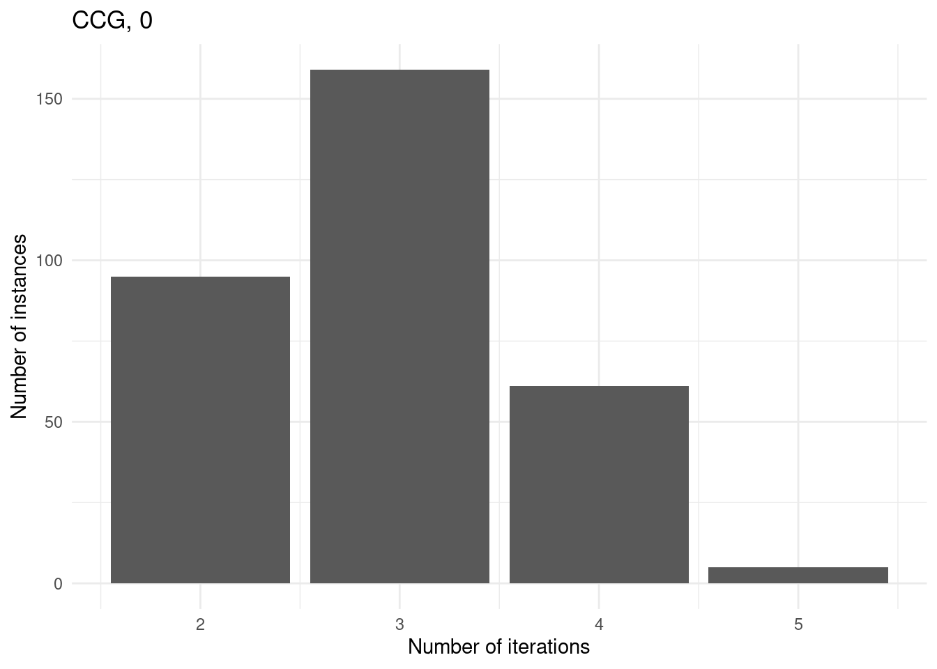
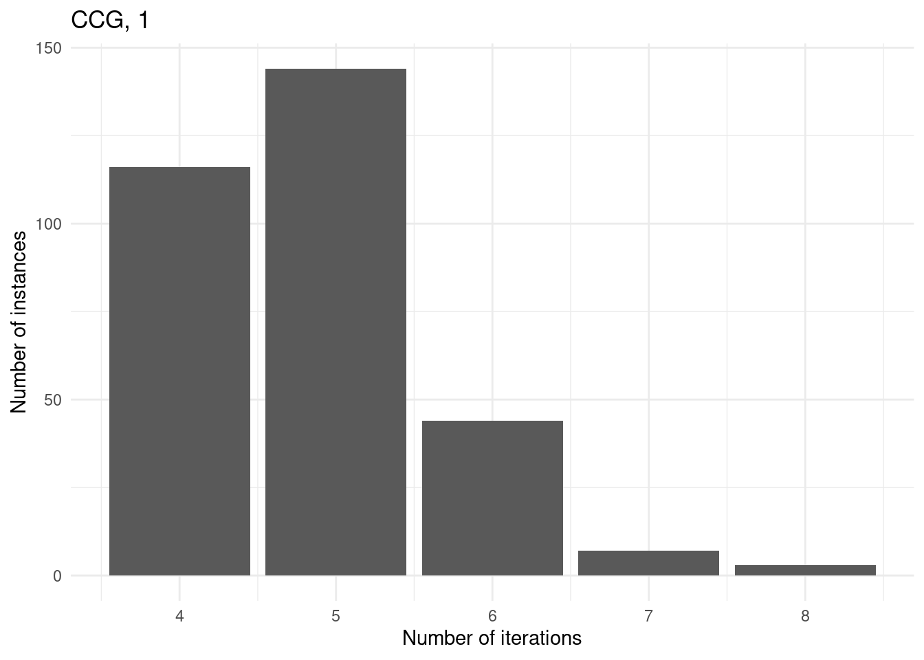
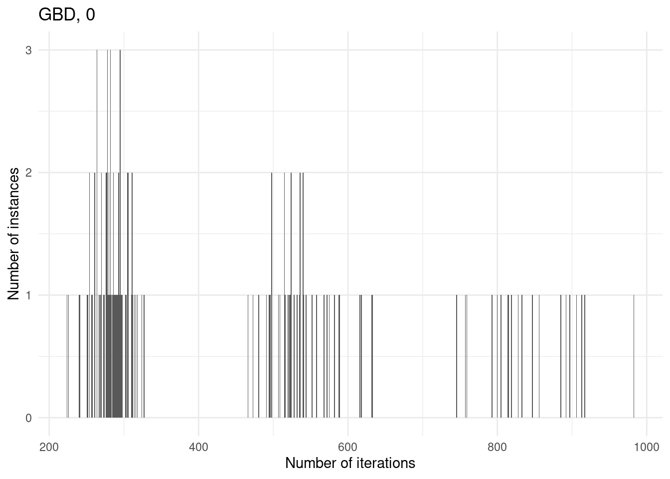
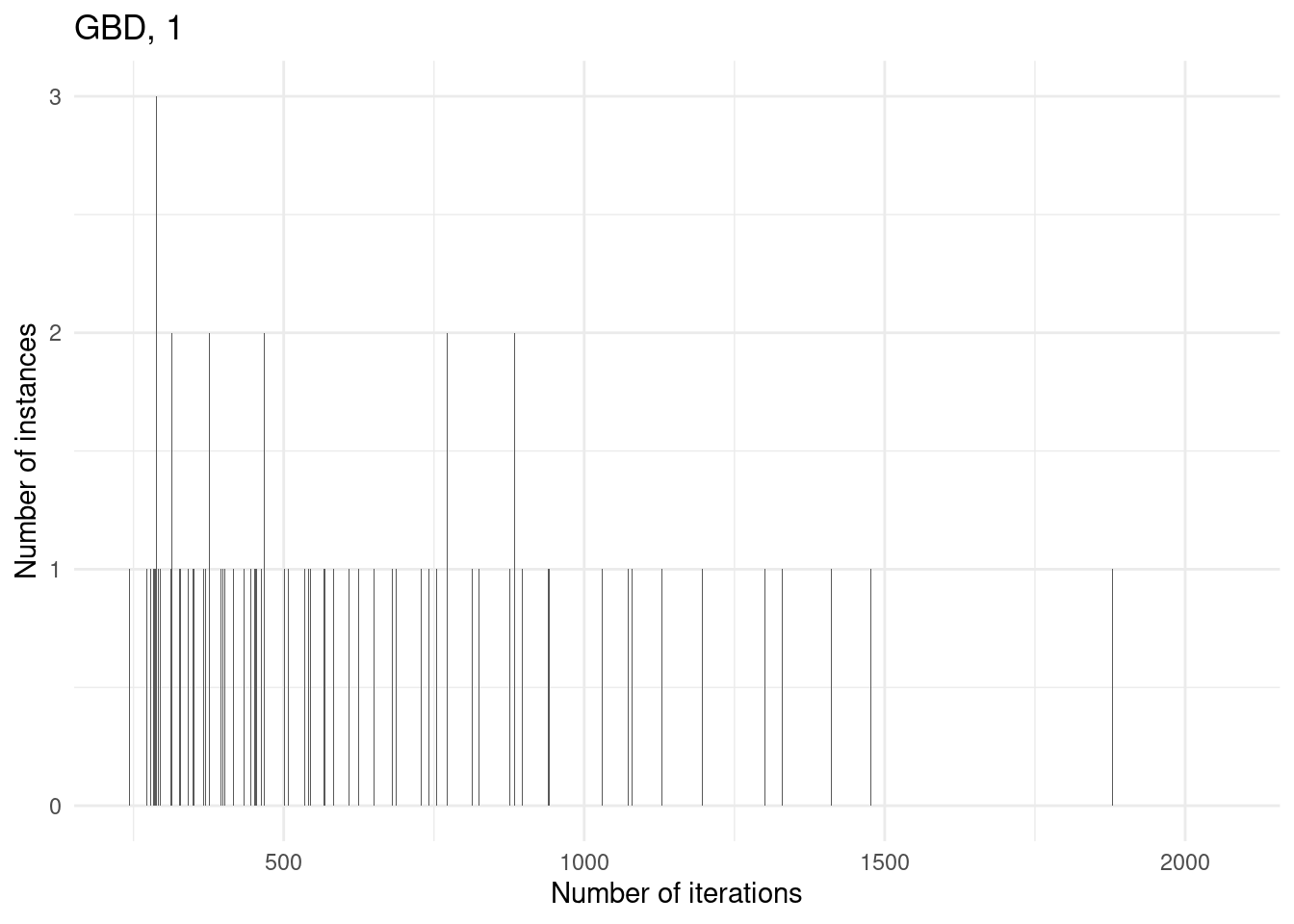
Number of iterations
for (method in unique(results$method_extended)) {

  p = ggplot(results[results$method_extended == method & results$unsolved == FALSE,], aes(x = iteration_count)) +
    geom_bar() +
    labs(
      title = method,
      x = "Number of iterations",
      y = "Number of instances"
    ) +
    theme_minimal()

  print(p)
}
This document is automatically generated after every
git push action on the public repository
hlefebvr/hlefebvr.github.io using rmarkdown and Github
Actions. This ensures the reproducibility of our data manipulation. The
last compilation was performed on the 12/09/24 14:05:40.