Table of content
Using column generation in constraint-and-column generation for adjustable robust optimization > FLP
Loading the data
Our results can be found in the results.flp.csv file
with the following columns:
- “tag”: a tag always equal to “result” used grep the result line in our execution log file.
- “instance”: the path to the instance.
- “standard_phase_time_limit”: the time limit for the standard phase (i.e., without using CG).
- “master_solver”: the solver used for solving the CCG master problem: STD for standard, i.e., Gurobi, CG for column generation.
- “status”: the final status.
- “reason”: the final status reason.
- “has_large_scaled”: true if the CG phase has been started, false otherwise.
- “n_iterations”: the number of iterations.
- “total_time”: the total time to solve the problem.
- “master_time”: the time spent solving the master problem.
- “adversarial_time”: the time spent solving the adversarial problem.
- “best_bound”: the best bound found.
- “best_obj”: the best feasible point value.
- “relative_gap”: the final relative gap.
- “absolute_gap”: the final absolute gap.
- “adversarial_unexpected_status”: the status of the adversarial problem solver if it is not Optimal.
- “with_heuristic”: true if the CG-based heuristic is used.
- “n_facilities”: the number of facilities in the instance.
- “n_customers”: the number of customers in the instance.
- “Gamma”: the value for the uncertainty budget \(\Gamma\).
- “blank”: this column is left blank.
data = read.csv("results.flp.csv", header = FALSE)
colnames(data) = c("tag", "instance", "standard_phase_time_limit", "master_solver", "status", "reason", "has_large_scaled", "n_iterations", "total_time", "master_time", "adversarial_time", "best_bound", "best_obj", "relative_gap", "absolute_gap", "adversarial_unexpected_status",  "with_heuristic", "n_facilities", "n_customers", "Gamma", "blank")
We start by removing the “tag” and the “blank” columns.
data = data[, !(names(data) %in% c("tag", "blank"))]We then remove instances which were not considered in our experimental results because none of the approaches could solve sufficiently many instances.
data = data[data$n_customers != 40,]
data = data[data$n_facilities == 10,]
For homogeneity, we fix the total_time of unsolved instances to the time limit.
data[data$total_time > 10800,]$total_time = 10800Then, we create a column named “method” which gives a specific name to each method, comprising the approach for solving the CCG master problem, the time limit of the standard phase and a flag indicating if the CG-based heuristic was used.
data$method = paste0(data$master_solver, "_TL", data$standard_phase_time_limit, "_H", data$with_heuristic)
unique(data$method)
## [1] "STD_TLInf_H0" "CG_TL60_H0" "CG_TL60_H1"data = data[data$method != "STD_TLInf_H1" & data$method != "CG_TL120_H0" & data$method != "CG_TL120_H1",]Our final data reads.
Empirical Cumulative Distribution Function (ECDF)
We plot the ECDF of computation time over our set of instances for all approaches.
ggplot(data, aes(x = total_time, col = method)) + stat_ecdf(pad = FALSE) +
  coord_cartesian(xlim = c(0,10800)) +
  theme_minimal()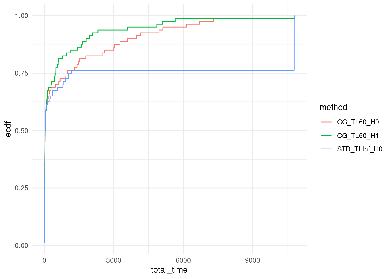
We export these results in csv to print them in tikz.
data_with_ecdf = data %>%
  group_by(method) %>%
  arrange(total_time) %>%
  mutate(ecdf_value = ecdf(total_time)(total_time)) %>%
  ungroup()

for (method in unique(data_with_ecdf$method)) {
  output = data_with_ecdf[data_with_ecdf$method == method,]
  output = output[,c("total_time", "ecdf_value")]
  output$log_total_time = log10(output$total_time)
  output = output[output$total_time < 10800,]
  write.csv(output, file = paste0(method, ".csv"), row.names = FALSE)
}
Summary table
In this section, we create a table summarizing the main outcome of our computational experiments.
We first focus on the solved instances.
summary_data_lt_10800 <- data %>%
  filter(total_time < 10800) %>%
  group_by(n_facilities, n_customers, Gamma, method) %>%
  summarize(
    avg_total_time = mean(total_time, na.rm = TRUE),
    avg_master_time = mean(master_time, na.rm = TRUE),
    avg_adversarial_time = mean(adversarial_time, na.rm = TRUE),
    avg_n_iterations = mean(n_iterations, na.rm = TRUE),
    sum_has_large_scaled = sum(has_large_scaled),
    num_lines = n(),
    .groups = "drop"
  ) %>%
  ungroup() %>%
  arrange(n_facilities, n_customers, Gamma, method)
Then, we compute averages over the unsolved instances.
summary_data_ge_10800 <- data %>%
  filter(total_time >= 10800) %>%
  group_by(n_facilities, n_customers, Gamma, method) %>%
  summarize(
    avg_n_iterations_unsolved = mean(n_iterations, na.rm = TRUE),
    num_lines_unsolved = n(),
    .groups = "drop"
  ) %>%
  ungroup() %>%
  arrange(n_facilities, n_customers, Gamma, method)
Finally, we merge our results.
transposed_data_lt_10800 <- summary_data_lt_10800 %>%
  pivot_wider(names_from = method, values_from = avg_total_time:num_lines)

transposed_data_ge_10800 <- summary_data_ge_10800 %>%
  pivot_wider(names_from = method, values_from = avg_n_iterations_unsolved:num_lines_unsolved) %>%
  select(-n_facilities, -n_customers, -Gamma)

cbind(
  transposed_data_lt_10800,
  transposed_data_ge_10800
) %>%
  kable() %>%
kable_styling(full_width = FALSE, position = "center")| n_facilities | n_customers | Gamma | avg_total_time_CG_TL60_H0 | avg_total_time_CG_TL60_H1 | avg_total_time_STD_TLInf_H0 | avg_master_time_CG_TL60_H0 | avg_master_time_CG_TL60_H1 | avg_master_time_STD_TLInf_H0 | avg_adversarial_time_CG_TL60_H0 | avg_adversarial_time_CG_TL60_H1 | avg_adversarial_time_STD_TLInf_H0 | avg_n_iterations_CG_TL60_H0 | avg_n_iterations_CG_TL60_H1 | avg_n_iterations_STD_TLInf_H0 | sum_has_large_scaled_CG_TL60_H0 | sum_has_large_scaled_CG_TL60_H1 | sum_has_large_scaled_STD_TLInf_H0 | num_lines_CG_TL60_H0 | num_lines_CG_TL60_H1 | num_lines_STD_TLInf_H0 | avg_n_iterations_unsolved_STD_TLInf_H0 | avg_n_iterations_unsolved_CG_TL60_H0 | avg_n_iterations_unsolved_CG_TL60_H1 | num_lines_unsolved_STD_TLInf_H0 | num_lines_unsolved_CG_TL60_H0 | num_lines_unsolved_CG_TL60_H1 |
|---|---|---|---|---|---|---|---|---|---|---|---|---|---|---|---|---|---|---|---|---|---|---|---|---|---|---|
| 10 | 20 | 2 | 730.2608 | 513.1331 | 77.63333 | 723.0262 | 505.7057 | 76.36180 | 7.171204 | 7.363157 | 1.222250 | 7.350000 | 7.350000 | 6.411765 | 5 | 5 | 0 | 20 | 20 | 17 | 7.000000 | NA | NA | 3 | NA | NA |
| 10 | 20 | 3 | 632.3732 | 461.4180 | 164.22367 | 623.3365 | 452.6818 | 163.03147 | 8.944192 | 8.646347 | 1.120693 | 9.789474 | 9.789474 | 8.800000 | 7 | 7 | 0 | 19 | 19 | 15 | 6.800000 | 26 | 27 | 5 | 1 | 1 |
| 10 | 30 | 2 | 1069.6240 | 439.6867 | 219.90575 | 1053.8821 | 423.8650 | 203.81612 | 15.655541 | 15.736596 | 16.014631 | 6.950000 | 6.950000 | 6.875000 | 9 | 9 | 0 | 20 | 20 | 16 | 4.750000 | NA | NA | 4 | NA | NA |
| 10 | 30 | 3 | 1115.9424 | 658.2883 | 79.38497 | 1097.9227 | 639.5282 | 69.34695 | 17.905963 | 18.647524 | 9.953583 | 8.650000 | 8.650000 | 7.615385 | 9 | 9 | 0 | 20 | 20 | 13 | 5.714286 | NA | NA | 7 | NA | NA |
This document is automatically generated after every
git push action on the public repository
hlefebvr/hlefebvr.github.io using rmarkdown and Github
Actions. This ensures the reproducibility of our data manipulation. The
last compilation was performed on the 12/09/24 14:05:54.