 Henri Lefebvre
Implementing Intersection Cuts for Mixed-Integer Bilevel Problems
Introduction
The cone defined by an LP basis
Problem statement
We consider a linear problem (LP) given in the form $$ \begin{aligned} \min_{\tilde{x}\in\mathbb{R}^n} \quad & c^\top \tilde{x} \\ \text{s.t.} \quad & \tilde{A} \tilde{x} \le b, \\ & \tilde{\ell} \le \tilde{x} \le \tilde{u}, \end{aligned} $$ with \(\tilde{A}\) the constraint matrix, \(b\) the right-hand side, \(c\) the objective coefficient vector and \(\tilde{\ell}\) and \(\tilde{u}\) the lower and upper bounds on the decision vector \(x\). In the following discusson, we also allow for \(\tilde{\ell}_j = -\infty\) or \( \tilde{u}_j = \infty \) for some \( j\in\{1,\dotsc,n\} \) in case some variables have no lower or no upper bound.
As classically done, we consider the standard form of this LP rather than its "natural" formulation stated above. The standard form is obtained by introducing slack variables \(s\) in such a way that all inequality constraints are turned into equality constraints. In our case, the LP in standard form reads $$ \begin{aligned} \min_{x,s} \quad & c^\top x \\ \text{s.t.} \quad & Ax + Is = b, \\ & \ell \le x \le u, \\ & s \ge 0. \end{aligned} $$ For the sake of presentation, we denote by \( A \) the matrix formed by appending the identity matrix \(I\) to the matrix \(\tilde{A}\), i.e., \( A := [\tilde{A},I] \). Additionally, \(\ell\) denotes the vector formed by appending \(m\) zeroes to the vector \(\tilde{\ell}\) and \(u\) denotes the vector formed by appending \(m\) infinite entries to the vector \(\tilde{u}\). With this notation, we study the LP written in standard and compact form $$ \begin{aligned} \min_x \quad & c^\top x \\ \text{s.t.} \quad & Ax = b, \\ & \ell \le x \le u. \end{aligned} $$ In the following, we define \( S := \{ 1,\dotsc,n \} \) the set of indices which corresponds to structural variables, i.e., non slack variables.
Recalls on the Simplex algorithm with bounded variables
Modern optimization solvers like Cplex typically solve LPs using the revised Simplex algorithm with bounded variables. This version of the Simplex explicitly accounts for bound constraints on the decision variables which is typically faster than treating them as standard constraints embedded in the definition of \(A\) and \(b\).
We say that a solution \( x^* \) is a basic solution if and only if the \(n+m\) components of \(x\) can be partitioned into \( (B,L,U) \) such that
- \( |B| = m \) and the matrix made of those columns in \( A \) whose index are in \(B\), noted \( A_B \), is invertible;
- It holds \( x_j^* = \ell_j \) for all \( j\in L \) and \(x_j^* = u_j\) for all \(j\in U\).
For more information on the Simplex algorithm with bounded variables, we refer to Chapter 8 of the book Linear Programming by V. Chvátal or to this YouTube video of R. Bixby (in particular starting at 6:44 "Issue 0: Bounds on Variables").
Computing the rays
Let \(x^*\) denote a basic feasible solution with partition \( (B,L,U) \). Then, one can express the basic variables in terms of the nonbasic ones by rewritting the system \( Ax = b \) as $$ \begin{aligned} Ax^* = b \iff & A_Bx_B^* + A_Lx_L^* + A_Ux_U^* = b \\ \iff & x_B^* = A_B^{-1}b - A_B^{-1}A_Lx_L^* - A_B^{-1}A_Ux_U^*. \end{aligned} $$ Recall from the Simplex algorithm that moving from one extreme point \( x^* \) to its neighboring extreme point, say \( x^k \), corresponds to a nonbasic variable entering the basis while a basic variable leaves the basis. Hence, pick any nonbasic variable (structural or slack) and let it enter the basis. To start with, let's assume that this variable has an index \( k\in L \). Because it is a nonbasic variable at its lower bound, making it entering the basis will lead to a positive change of the form \( x_k^k \gets x_k^* + \xi \) for some \( \xi > 0 \) while other nonbasic variables do not change. More formally, performing a pivot operation leads to $$ \begin{array}{cl} x_B^k &= A_B^{-1}b - A_B^{-1}(A_{L\backslash\{k\}}x_{L\backslash\{k\}}^* + A_k(x_k^* + \xi) ) - A_B^{-1}A_Ux_U^*, \\ x_k^k &= x_k^* + \xi, \\ x_{L\backslash\{k\}}^k &= x_{L\backslash\{k\}}^*, \\ x_U^k &= x_U^*. \end{array} $$ for some \( \xi > 0 \).
The ray associated to moving from the basic solution \(x^*\) to the nonbasic solution \(x^k\) can be computed as \( r^k := x^k - x^* \). Hence, we obtain $$ \begin{array}{cl} r^k_B &= -A_B^{-1}A_k\xi, \\ r_k^k &= \xi, \\ r_{L\backslash\{k\}}^k &= 0, \\ r_U &= 0, \end{array} $$ for some \( \xi > 0 \). Note that, for any \( \xi \), this ray is colinear to the ray $$ \begin{array}{cl} r^k_B &= -A_B^{-1}A_k, \\ r_k^k &= 1, \\ r_{L\backslash\{k\}}^k &= 0, \\ r_U &= 0. \end{array} $$ By convention, we will consider the latter in our implementation. Similarly, if the nonbasic variable which we select to enter the basis is at its upper bound, i.e., if \(k\in U\), one obtains the ray $$ \begin{array}{cl} r^k_B &= A_B^{-1}A_k, \\ r_k^k &= -1, \\ r_{U\backslash\{k\}}^k &= 0, \\ r_L &= 0. \end{array} $$ Notice how the sign flipped due to the change \( x_k^k \gets x_k^* - \xi \) for some \( \xi> 0 \) instead of \( x_k^k \gets x_k^* + \xi \). This is because \(x_k\) is at its upper bound and can only decrease its value to preserve feasibility.
Question for later: What about fixed variables?Computing intersection cuts
From the previous section, we are now able to compute the description of a cone which is pointed at \( x^* \) and which contains all feasible points, i.e., we have $$ C := \left\{ x^* + \sum_{k\in L\cup U} \lambda_k r^k : \lambda_k \ge 0 \text{ for all }k\in L\cup U \right\}. $$ In this section, we assume to know the description of a polyhedron \( S \) which contains \( x^* \) in its interior but no feasible point for the original problem. We assume that this description is given by $$ S := \left\{ x : Fx \ge g \right\}. $$ The intersection cut is defined as the halfspace \( \alpha^\top x \le \beta \) whose boundary contains all intersection points between the cone \( C \) and the set \( S \). Hence, our first task is to compute these points. Hence, for each ray \( r^k \) with \( k\in L\cup U \), we want to solve $$ \begin{aligned} \max_{\lambda_k} \quad & \lambda_k \\ \text{s.t.} \quad & x^* + \lambda_kr^k \in S, \\ & \lambda_k \ge 0. \end{aligned} $$ This problem can be solved analytically by noting the following: $$ \begin{aligned} F(x^* + \lambda_kr^k) \ge g & \iff \lambda_k (Fr^k) \ge g - Fx^* \\ & \iff \begin{cases} \lambda_k \ge (g_i - F_{i\cdot}x^*)/(F_{i\cdot}r^k) & \text{if } F_{i\cdot}r^k > 0, \\ \lambda_k \le (g_i - F_{i\cdot}x^*)/(F_{i\cdot}r^k) & \text{if } F_{i\cdot}r^k < 0, \\ \lambda_k \ge 0 & \text{otherwise}, \end{cases} \\ & \iff \lambda_k = \min_{i} \left\{ (g_i - F_{i\cdot}x^*)/(F_{i\cdot}r^k) : F_{i\cdot}r^k \le 0 \right\}. \end{aligned} $$ Note that if \( F_{i\cdot}r^k \ge 0 \) for all \( i \), we fix \( \lambda_k = \infty \). This situation corresponds to a case in which \( r^k \) is parallel to a face of \( C \).
The coefficients \( (\alpha, \beta) \) of the intersection cut are then given by the solution to the following linear system: $$ \begin{aligned} & \alpha^\top( x^* + \lambda_kr^k ) = \beta & \text{for all } k\in L\cup U : \lambda_k < \infty, \\ & \alpha^\top r^k = 0 & \text{for all } k\in L\cup U : \lambda_k = \infty. \end{aligned} $$ The first set of constraints ask that the boundary of the halfspace contains the intersection points while the second set of constraints requires that the boundary is parallel to the extreme rays \(r^k\) if no intersection point exists.
Here again, an analytical solution can be obtained. Note that there are \( n + 1 \) variables and \( |L\cup U| = n \) constraints. Hence, there is a unique solution (up to a constant) as the extreme rays \( r^k \) are linearly independent. For the example, let's consider \( k\in L \) such that \( \lambda_k < \infty \). We rewrite the \( k \)-th constraint as $$ \begin{aligned} & \alpha^\top( x^* + \lambda_k r^k ) = \beta \\ \iff & \alpha_{B}^\top ( x^*_{B} + \lambda_k r^k_{B} ) + \alpha_{L}^\top ( x^*_{L} + \lambda_k r^k_{L} ) + \alpha_{U}^\top ( x^*_{U} + \lambda_k r^k_{U} ) = \beta \\ \iff & \alpha_{B}^\top ( A_B^{-1}b - A_B^{-1}A_L\ell_L - A_B^{-1}A_Uu_U - \lambda_k A^{-1}_BA_k ) + \lambda_k\alpha_k = \beta \\ \iff & \alpha_k = \frac{\beta - \alpha_{B}^\top ( A_B^{-1}b - A_B^{-1}A_L\ell_L - A_B^{-1}A_Uu_U )}{\lambda_k} - \lambda_k\alpha_B^\top A^{-1}_BA_k \end{aligned} $$
Intersection cuts for mixed-integer bilevel problems
The Moore and Bard example
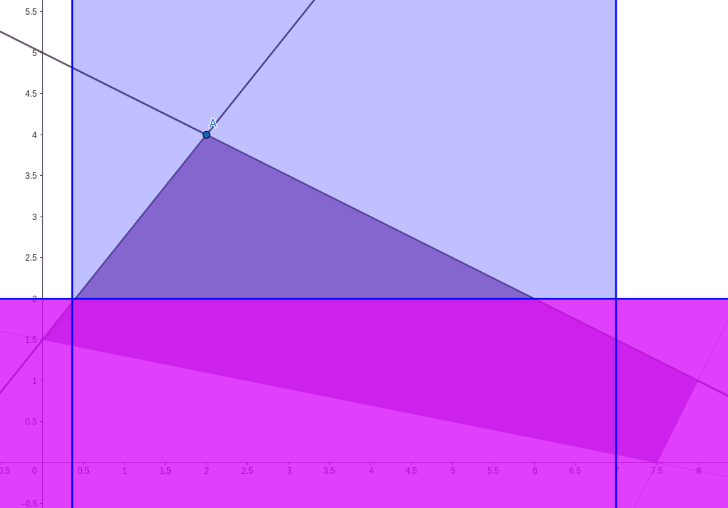
We consider a toy LP which has two (structural) variables and that is given by $$ \begin{aligned} \min_{x,y} \quad & -x - 10y \\ \text{s.t.} \quad & -25x + 20y \le 30, \\ & x + 2y \le 10, \\ & 2x - y \le 15, \\ & 2x + 10y \ge 15, \\ & x,y \ge 0. \end{aligned} $$ This example actually stems from a famous bilevel problem considered by Moore and Bard (1990) and corresponds to the linear relaxation of its high-point relaxation.
The feasible region of our example and its optimal point can be
represented in the following two-dimensional plot.
The optimal point is \( (x^*,y^*) \) and is associated to the following simplex tableau.
| \(x\) | \(y\) | \(s_1\) | \(s_2\) | \(s_3\) | \(s_4\) | |
|---|---|---|---|---|---|---|
| \(x\) | 1 | 0 | -0.0286 | 0.2857 | 0 | 0 |
| \(y\) | 0 | 1 | 0.0143 | 0.3571 | 0 | 0 |
| \(s_3\) | 0 | 0 | 0.0714 | -0.2143 | 1 | 0 |
| \(s_4\) | 0 | 0 | 0.0857 | 4.1429 | 0 | 1 |
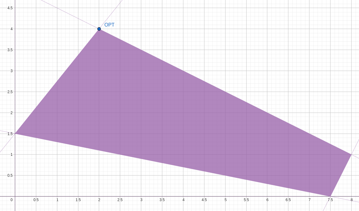
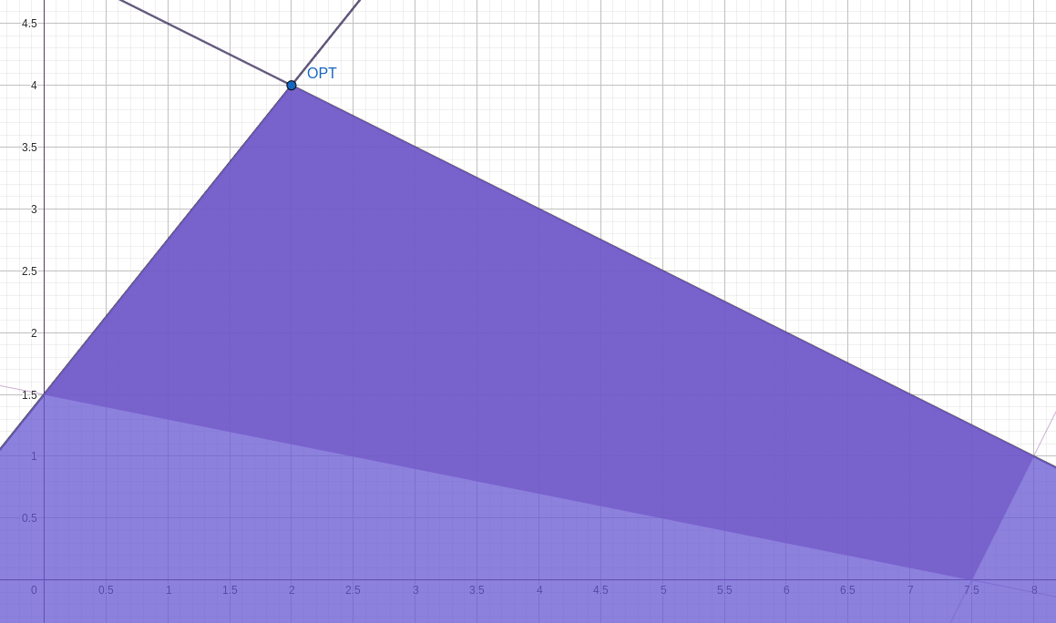
A graphical representation of this cone is given hereafter.
Implemetation in Cplex
Defining the high-point relaxation
#define CALL_CPLEX(stmt) \
if (int status = stmt ; status) { \
    throw std::runtime_error("CPLEX error from C API, " \
            "call ended with status " + std::to_string(status)); \
}
int status;
CPXENVptr env = CPXopenCPLEX(&status);
CPXLPptr lp = CPXcreateprob(env, &status, "model");

// Set objective sense
CALL_CPLEX(CPXchgobjsen(env, lp, CPX_MIN))

// Add variables: x and y
const int numcols = 2;
const std::vector<char> coltypes { 'I', 'I' };
const std::vector<double> obj { -1.0, -10.0 };
const std::vector<double> lb { 1, 0.0 };
const std::vector<double> ub { 10, 10 };
std::vector<char*> colnames { const_cast<char*>("x"),
                              const_cast<char*>("y") };

CALL_CPLEX(CPXnewcols(env,
                      lp,
                      numcols,
                      obj.data(),
                      lb.data(),
                      ub.data(),
                      coltypes.data(),
                      colnames.data()))

// Add constraints
// Constraint coefficients
const std::vector<int> rmatbeg  {0, 2, 4, 6};
const std::vector<int> rmatind {
        0, 1,   // -25x + 20y
        0, 1,   //  x  + 2y
        0, 1,   //  2x -  y
        0, 1    //  2x + 10y
};
const std::vector<double> rmatval {
        -25, 20,
        1,   2,
        2,  -1,
        2,  10
};
const std::vector<char> ctr_type { 'L', 'L', 'L', 'G' };
const std::vector<double> rhs { 30, 10, 15, 15 };
std::vector<char*> rownames {
        const_cast<char*>("c1"),
        const_cast<char*>("c2"),
        const_cast<char*>("c3"),
        const_cast<char*>("c4")
};

CALL_CPLEX(CPXaddrows(
        env,
        lp,
        0,
        4,
        rmatval.size(),
        rhs.data(),
        ctr_type.data(),
        rmatbeg.data(),
        rmatind.data(),
        rmatval.data(),
        nullptr,
        rownames.data()
))
Computing the cone defined by an LP basis
// Get number of column and rows
const int n_cols = CPXgetnumcols(env, lp);
const int n_rows = CPXgetnumrows(env, lp);

// Get row sense
std::vector<char> row_sense(n_rows);
CALL_CPLEX(CPXgetsense(env, lp, row_sense.data(), 0, n_rows - 1))

// Get variable lower bounds
std::vector<double> col_lb(n_cols);
CALL_CPLEX(CPXgetlb(env, lp, col_lb.data(), 0, n_cols - 1))

// Get variable upper bounds
std::vector<double> col_ub(n_cols);
CALL_CPLEX(CPXgetub(env, lp, col_ub.data(), 0, n_cols - 1))
// Get the current LP basis
std::vector<int> var_status(n_cols), row_status(n_rows);
CALL_CPLEX(CPXgetbase(env, lp, var_status.data(), row_status.data()))// Get basis indices
std::vector<int> basis_indices(n_basic_variables);
std::vector<double> x_basis(n_basic_variables);
CALL_CPLEX(CPXgetbhead(env, lp, basis_indices.data(), x_basis.data()))// Get non-basic variable indices
std::vector<int> non_basic_variable_indices;
for (unsigned int j = 0 ; j < n_cols ; ++j) {
if (var_status[j] != CPX_BASIC) {
non_basic_variable_indices.emplace_back(j);
}
}
// Get non-basic slack variable indices
for (unsigned int i = 0 ; i < n_rows ; ++i) {
if (row_status[i] != CPX_BASIC) {
non_basic_variable_indices.emplace_back(- i - 1);
}
}const unsigned int n_non_basic_variables = non_basic_variable_indices.size();
const unsigned int n_basic_variables = n_cols + n_rows - n_non_basic_variables;
// Compute rays
std::vector<std::vector<double>> rays(n_non_basic_variables,
    std::vector<double>(n_cols, 0.0)
);
for (unsigned int j = 0 ; j < n_non_basic_variables ; ++j) {

    const int j_index = non_basic_variable_indices[j];

    double coeff;
    if (j_index >= 0) {
        assert(var_status[j_index] != CPX_FREE_SUPER);
        if (var_status[j_index] == CPX_AT_UPPER) {
            rays[j][j_index] = - 1.0;
            coeff = 1.0;
        } else {
            rays[j][j_index] = + 1.0;
            coeff = -1.0;
        }
    } else {
        assert(row_status[j_index] != CPX_FREE_SUPER);
        if (row_sense[-j_index - 1] == 'G') {
            coeff = 1.0;
        } else {
            coeff = -1.0;
        }
    }

    std::vector<double> BinvAj(n_rows);
    CALL_CPLEX(CPXbinvacol(env, lp, j_index, BinvAj.data()))

    for (unsigned int k = 0 ; k < n_basic_variables ; ++k) {

        const int k_index = basis_indices[k];
        if (k_index >= 0) {
            rays[j][k_index] = coeff * BinvAj[k];
        }

    }

}