Using column generation in constraint-and-column generation for adjustable robust optimization > FLP
Loading the data
Our results can be found in the results.flp.csv file
with the following columns:
- “tag”: a tag always equal to “result” used grep the result line in our execution log file.
- “instance”: the path to the instance.
- “standard_phase_time_limit”: the time limit for the standard phase (i.e., without using CG).
- “master_solver”: the solver used for solving the CCG master problem: STD for standard, i.e., Gurobi, CG for column generation.
- “status”: the final status.
- “reason”: the final status reason.
- “has_large_scaled”: true if the CG phase has been started, false otherwise.
- “n_iterations”: the number of iterations.
- “total_time”: the total time to solve the problem.
- “master_time”: the time spent solving the master problem.
- “adversarial_time”: the time spent solving the adversarial problem.
- “best_bound”: the best bound found.
- “best_obj”: the best feasible point value.
- “relative_gap”: the final relative gap.
- “absolute_gap”: the final absolute gap.
- “adversarial_unexpected_status”: the status of the adversarial problem solver if it is not Optimal.
- “with_heuristic”: true if the CG-based heuristic is used.
- “n_facilities”: the number of facilities in the instance.
- “n_customers”: the number of customers in the instance.
- “Gamma”: the value for the uncertainty budget \(\Gamma\).
- “blank”: this column is left blank.
data = rbind(
  read.csv("results.csv", header = FALSE)
)
colnames(data) = c("slurm_file", "tag", "instance", "standard_phase_time_limit_raw", "Gamma", "with_heuristic", "standard_phase_time_limit", "master_solver", "status", "reason", "has_large_scaled", "n_iterations", "total_time", "master_time", "adversarial_time", "best_bound", "best_obj", "relative_gap", "absolute_gap", "second_stage.mean", "second_stage.std_dev", "adversarial_unexpected_status", "memory_used", "memory_limit")
data = data %>% mutate(instance = basename(instance),
                n_facilities = as.numeric(sub(".*F(\\d+)_C.*", "\\1", instance)),
                n_customers = as.numeric(sub(".*C(\\d+)_.*", "\\1", instance))
                )
We start by removing the “tag” and the “blank” columns.
#data = data[, !(names(data) %in% c("tag", "blank"))]We then remove instances which were not considered in our experimental results because none of the approaches could solve sufficiently many instances.
#data = data[data$n_customers != 40,]
#data = data[data$n_facilities == 10,]
For homogeneity, we fix the total_time of unsolved instances to the time limit.
if (sum(data$tag == "iteration") > 0 ) {
  data[data$tag == "iteration",]$total_time = 10800
}

if (sum(data$total_time > 10800) > 0 ) {
  data[data$total_time > 10800,]$total_time = 10800
}
Then, we create a column named “method” which gives a specific name to each method, comprising the approach for solving the CCG master problem, the time limit of the standard phase and a flag indicating if the CG-based heuristic was used.
data$method = paste0(data$master_solver, "_TL", data$standard_phase_time_limit, "_H", data$with_heuristic)
unique(data$method)
## [1] "CG_TL0_Hfalse" "CG_TL0_Htrue" "STD_TLInf_Hfalse"data = data[data$method != "STD_TLInf_H1" & data$method != "CG_TL120_H0" & data$method != "CG_TL120_H1",]Our final data reads.
Sanity Check
# Define the relative tolerance
tolerance <- 10^-2

# Filter the data where time < 10800 and group by 'instance'
validation <- data %>%
  filter(total_time < 10800) %>%
  group_by(paste0(instance, "_", Gamma)) %>%
  summarise(min_best_obj = min(best_obj), max_best_obj = max(best_obj)) %>%
  mutate(valid = abs(max_best_obj - min_best_obj) / max(abs(min_best_obj), 1) <= tolerance)

# Check if all instances are valid
if (all(validation$valid)) {
  print("All methods find the same best_obj value within the relative tolerance for all instances.")
} else {
  print("Methods do not find the same best_obj value within the relative tolerance for some instances.")
  print(validation %>% filter(!valid))  # Show the instances that failed validation
}
## [1] "All methods find the same best_obj value within the relative tolerance for all instances."Empirical Cumulative Distribution Function (ECDF)
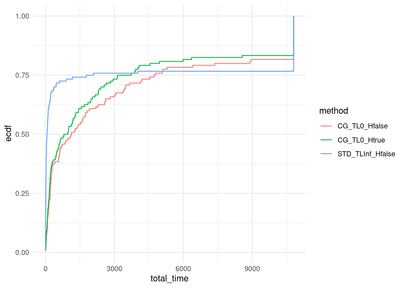
We plot the ECDF of computation time over our set of instances for all approaches.
ggplot(data, aes(x = total_time, col = method)) + stat_ecdf(pad = FALSE) +
  coord_cartesian(xlim = c(0,10800)) +
  # scale_x_log10() +
  theme_minimal()
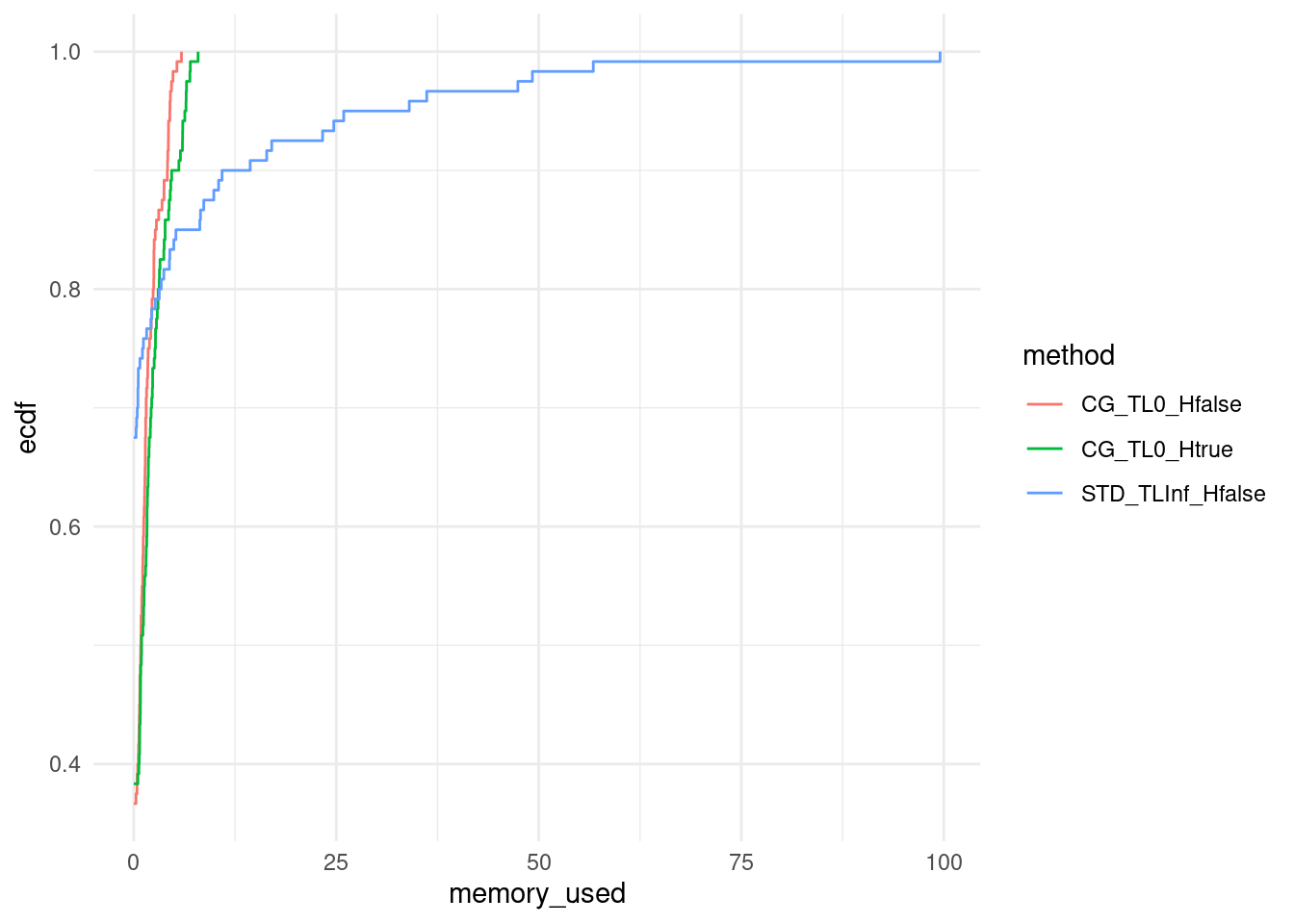
ggplot(data, aes(x = memory_used, col = method)) +
  stat_ecdf(pad = FALSE) +
  theme_minimal()
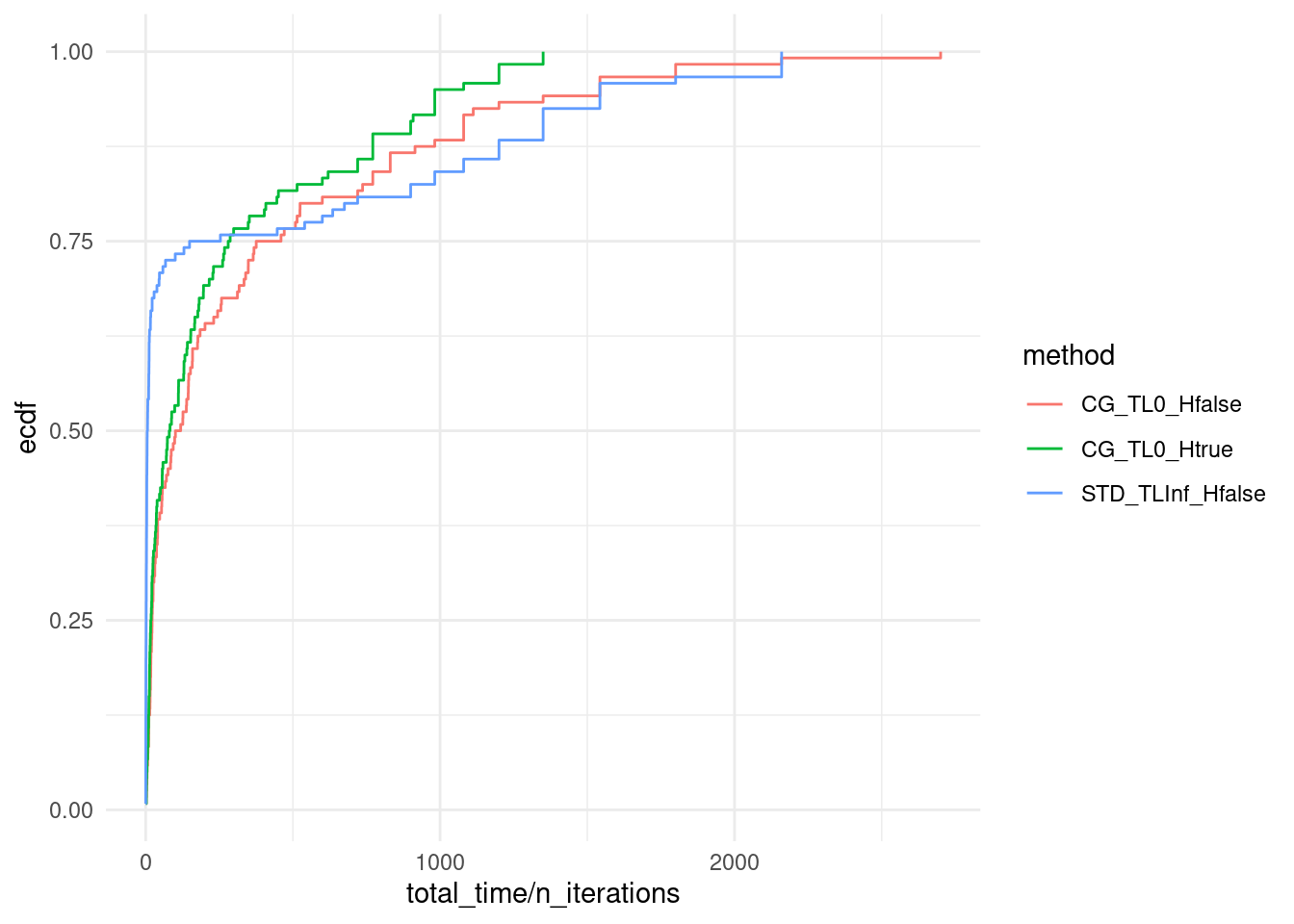
ggplot(data, aes(x = total_time / n_iterations, col = method)) + stat_ecdf(pad = FALSE) +
  # scale_x_log10() +
  theme_minimal()
We export these results in csv to print them in tikz.
#data_with_ecdf = data %>%
#  group_by(method) %>%
#  arrange(total_time) %>%
#  mutate(ecdf_value = ecdf(total_time)(total_time)) %>%
#  ungroup()

n_points <- 1000
x_points <- seq(1, 10800, length.out = n_points)

data_with_ecdf <- data %>%
  group_by(method) %>%
  arrange(total_time) %>%
  group_modify(~ {
    # Create ECDF function for the current method
    ecdf_func <- ecdf(.x$total_time)
    # Compute ECDF values for the specified points
    tibble(total_time = x_points, ecdf_value = 100 * ecdf_func(x_points))
  }) %>%
  ungroup()

for (method in unique(data_with_ecdf$method)) {
  output = data_with_ecdf[data_with_ecdf$method == method,]
  output = output[,c("total_time", "ecdf_value")]
  output = output[output$total_time < 10800,]
  write.csv(output, file = paste0("TIME_", method, ".csv"), row.names = FALSE)
}
n_points <- 1000
x_points <- seq(1, 100, length.out = n_points)
data_with_ecdf <- data %>%
group_by(method) %>%
arrange(memory_used) %>%
group_modify(~ {
# Create ECDF function for the current method
ecdf_func <- ecdf(.x$memory_used)
# Compute ECDF values for the specified points
tibble(memory_used = x_points, ecdf_value = 100 * ecdf_func(x_points))
}) %>%
ungroup()
for (method in unique(data_with_ecdf$method)) {
output = data_with_ecdf[data_with_ecdf$method == method,]
output = output[,c("memory_used", "ecdf_value")]
write.csv(output, file = paste0("MEMORY_", method, ".csv"), row.names = FALSE)
}Summary table
In this section, we create a table summarizing the main outcome of our computational experiments.
We first focus on the solved instances.
summary_data_lt_10800 <- data %>%
  filter(total_time < 10800) %>%
  group_by(n_facilities, n_customers, Gamma, method) %>%
  summarize(
    avg_total_time = mean(total_time, na.rm = TRUE),
    avg_master_time = mean(master_time, na.rm = TRUE),
    avg_adversarial_time = mean(adversarial_time, na.rm = TRUE),
    avg_n_iterations = mean(n_iterations, na.rm = TRUE),
    sum_has_large_scaled = sum(has_large_scaled),
    sum_oom = sum(tag == "iteration"),
    num_lines = n(),
    .groups = "drop"
  ) %>%
  ungroup() %>%
  arrange(n_facilities, n_customers, Gamma, method)
Then, we compute averages over the unsolved instances.
summary_data_ge_10800 <- data %>%
  filter(total_time >= 10800) %>%
  group_by(n_facilities, n_customers, Gamma, method) %>%
  summarize(
    avg_n_iterations_unsolved = mean(n_iterations, na.rm = TRUE),
    num_lines_unsolved = n(),
    .groups = "drop"
  ) %>%
  ungroup() %>%
  arrange(n_facilities, n_customers, Gamma, method)
Finally, we merge our results.
transposed_data_lt_10800 <- summary_data_lt_10800 %>%
  pivot_wider(names_from = method, values_from = avg_total_time:num_lines)

transposed_data_ge_10800 <- summary_data_ge_10800 %>%
  pivot_wider(names_from = method, values_from = avg_n_iterations_unsolved:num_lines_unsolved)

transposed_data_lt_10800 %>% kable()| n_facilities | n_customers | Gamma | avg_total_time_CG_TL0_Hfalse | avg_total_time_CG_TL0_Htrue | avg_total_time_STD_TLInf_Hfalse | avg_master_time_CG_TL0_Hfalse | avg_master_time_CG_TL0_Htrue | avg_master_time_STD_TLInf_Hfalse | avg_adversarial_time_CG_TL0_Hfalse | avg_adversarial_time_CG_TL0_Htrue | avg_adversarial_time_STD_TLInf_Hfalse | avg_n_iterations_CG_TL0_Hfalse | avg_n_iterations_CG_TL0_Htrue | avg_n_iterations_STD_TLInf_Hfalse | sum_has_large_scaled_CG_TL0_Hfalse | sum_has_large_scaled_CG_TL0_Htrue | sum_has_large_scaled_STD_TLInf_Hfalse | sum_oom_CG_TL0_Hfalse | sum_oom_CG_TL0_Htrue | sum_oom_STD_TLInf_Hfalse | num_lines_CG_TL0_Hfalse | num_lines_CG_TL0_Htrue | num_lines_STD_TLInf_Hfalse |
|---|---|---|---|---|---|---|---|---|---|---|---|---|---|---|---|---|---|---|---|---|---|---|---|
| 10 | 20 | 3 | 417.7230 | 513.5151 | 19.865948 | 412.3643 | 508.2297 | 15.105566 | 2.627364 | 2.560662 | 2.787303 | 9.400000 | 9.400000 | 9.400000 | 10 | 10 | 0 | 0 | 0 | 0 | 10 | 10 | 10 |
| 10 | 20 | 4 | 178.5199 | 172.0768 | 7.292702 | 174.7246 | 168.4561 | 3.936395 | 2.588857 | 2.498928 | 2.483051 | 7.600000 | 7.600000 | 7.600000 | 10 | 10 | 0 | 0 | 0 | 0 | 10 | 10 | 10 |
| 10 | 30 | 3 | 464.5931 | 416.2975 | 44.760516 | 451.5422 | 402.4616 | 32.211216 | 9.708875 | 10.349557 | 9.649474 | 8.200000 | 8.200000 | 8.200000 | 10 | 10 | 0 | 0 | 0 | 0 | 10 | 10 | 10 |
| 10 | 30 | 4 | 634.1579 | 558.3903 | 40.784240 | 616.6238 | 540.1934 | 23.700220 | 11.872204 | 12.941370 | 12.648772 | 12.700000 | 12.700000 | 12.800000 | 10 | 10 | 0 | 0 | 0 | 0 | 10 | 10 | 10 |
| 10 | 40 | 3 | 664.4191 | 481.2485 | 67.691217 | 626.2877 | 444.4605 | 45.310576 | 28.340392 | 27.441523 | 18.328150 | 9.100000 | 9.100000 | 9.375000 | 10 | 10 | 0 | 0 | 0 | 0 | 10 | 10 | 8 |
| 10 | 40 | 4 | 851.3128 | 744.6359 | 23.939155 | 803.8878 | 693.2411 | 15.397536 | 31.404191 | 33.905961 | 6.468526 | 10.500000 | 10.500000 | 9.125000 | 10 | 10 | 0 | 0 | 0 | 0 | 10 | 10 | 8 |
| 15 | 20 | 3 | 1155.3760 | 909.2798 | 501.899811 | 1136.9408 | 891.4251 | 484.597658 | 14.185783 | 14.006380 | 14.844869 | 9.555556 | 9.500000 | 9.333333 | 9 | 10 | 0 | 0 | 0 | 0 | 9 | 10 | 9 |
| 15 | 20 | 4 | 2618.4744 | 2497.9198 | 107.368886 | 2580.1352 | 2460.9833 | 77.077313 | 30.054111 | 29.618341 | 26.871270 | 11.444444 | 11.444444 | 10.285714 | 9 | 9 | 0 | 0 | 0 | 0 | 9 | 9 | 7 |
| 15 | 30 | 3 | 2541.2373 | 1905.3680 | 383.903583 | 2444.4947 | 1741.6952 | 282.878900 | 80.371847 | 147.827033 | 83.786755 | 9.500000 | 9.500000 | 10.500000 | 6 | 6 | 0 | 0 | 0 | 0 | 6 | 6 | 6 |
| 15 | 30 | 4 | 4010.2900 | 2862.4740 | 566.983560 | 3856.0360 | 2702.8180 | 442.687620 | 133.368914 | 139.062352 | 109.213804 | 12.000000 | 12.400000 | 12.400000 | 5 | 5 | 0 | 0 | 0 | 0 | 5 | 5 | 5 |
| 15 | 40 | 3 | 5372.7780 | 3714.3450 | 183.896200 | 5280.0640 | 3551.7100 | 93.029740 | 84.230000 | 152.602750 | 85.707840 | 9.200000 | 8.833333 | 9.200000 | 5 | 6 | 0 | 0 | 0 | 0 | 5 | 6 | 5 |
| 15 | 40 | 4 | 4376.4425 | 2583.5400 | 995.068267 | 4103.1275 | 2315.2800 | 639.099533 | 235.037450 | 230.214125 | 307.095133 | 8.500000 | 9.000000 | 8.333333 | 4 | 4 | 0 | 0 | 0 | 0 | 4 | 4 | 3 |
transposed_data_ge_10800 %>% kable()| n_facilities | n_customers | Gamma | avg_n_iterations_unsolved_STD_TLInf_Hfalse | avg_n_iterations_unsolved_CG_TL0_Hfalse | avg_n_iterations_unsolved_CG_TL0_Htrue | num_lines_unsolved_STD_TLInf_Hfalse | num_lines_unsolved_CG_TL0_Hfalse | num_lines_unsolved_CG_TL0_Htrue |
|---|---|---|---|---|---|---|---|---|
| 10 | 40 | 3 | 5.500000 | NA | NA | 2 | NA | NA |
| 10 | 40 | 4 | 9.000000 | NA | NA | 2 | NA | NA |
| 15 | 20 | 3 | 11.000000 | 5.000000 | NA | 1 | 1 | NA |
| 15 | 20 | 4 | 11.666667 | 15.000000 | 15.00000 | 3 | 1 | 1 |
| 15 | 30 | 3 | 12.500000 | 13.500000 | 14.25000 | 4 | 4 | 4 |
| 15 | 30 | 4 | 13.800000 | 13.200000 | 13.40000 | 5 | 5 | 5 |
| 15 | 40 | 3 | 7.200000 | 7.600000 | 10.00000 | 5 | 5 | 4 |
| 15 | 40 | 4 | 7.857143 | 8.833333 | 11.16667 | 7 | 6 | 6 |
#cbind(
#  transposed_data_lt_10800,
#  transposed_data_ge_10800
#) %>%
#  kable() %>%
#  kable_styling(full_width = FALSE, position = "center")
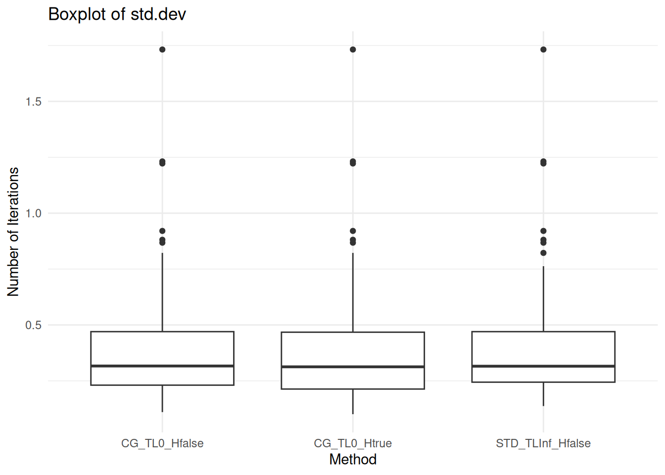
Second-stage Deviations
ggplot(data, aes(x = method, y = second_stage.std_dev / abs(second_stage.mean))) +
  geom_boxplot() +
  labs(title = "Boxplot of std.dev",
       x = "Method",
       y = "Number of Iterations") +
  theme_minimal()
git push action on the public repository
hlefebvr/hlefebvr.github.io using rmarkdown and Github
Actions. This ensures the reproducibility of our data manipulation. The
last compilation was performed on the 05/03/26 11:03:32.
 Henri Lefebvre