 Henri Lefebvre
Using column generation in constraint-and-column generation for adjustable robust optimization > JSP
Loading the data
Our results can be found in the results.jsp.csv file
with the following columns:
- “tag”: a tag always equal to “result” used grep the result line in our execution log file.
- “instance”: the path to the instance.
- “standard_phase_time_limit”: the time limit for the standard phase (i.e., without using CG).
- “master_solver”: the solver used for solving the CCG master problem: STD for standard, i.e., Gurobi, CG for column generation.
- “status”: the final status.
- “reason”: the final status reason.
- “has_large_scaled”: true if the CG phase has been started, false otherwise.
- “n_iterations”: the number of iterations.
- “total_time”: the total time to solve the problem.
- “master_time”: the time spent solving the master problem.
- “adversarial_time”: the time spent solving the adversarial problem.
- “best_bound”: the best bound found.
- “best_obj”: the best feasible point value.
- “relative_gap”: the final relative gap.
- “absolute_gap”: the final absolute gap.
- “adversarial_unexpected_status”: the status of the adversarial problem solver if it is not Optimal.
- “with_heuristic”: true if the CG-based heuristic is used.
- “with_non_optimal_pricing”: always false.
- “n_jobs”: the number of jobs in the instance.
- “Gamma”: the value for the uncertainty budget \(\Gamma\).
- “blank”: this column is left blank.
data = rbind(
  read.csv("results-filtered.csv", header = FALSE)
)
colnames(data) = c("slurm_file", "tag", "instance", "standard_phase_time_limit_raw", "Gamma", "with_heuristic", "standard_phase_time_limit", "master_solver", "status", "reason", "has_large_scaled", "n_iterations", "total_time", "master_time", "adversarial_time", "best_bound", "best_obj", "relative_gap", "absolute_gap", "second_stage.mean", "second_stage.std_dev", "adversarial_unexpected_status", "memory_used", "memory_limit")
#write.csv(data %>% filter(Gamma %in% c(3,6)), "results-filtered.csv", row.names = FALSE, col.names = FALSE)
data = data %>% mutate(instance = basename(instance),
                n_jobs = as.numeric(sub(".*N(\\d+)_R.*", "\\1", instance))
                )
We start by removing the “tag” and the “blank” columns.
#data = data[, !(names(data) %in% c("tag", "blank"))]For homogeneity, we fix the total_time of unsolved instances to the time limit.
if (sum(data$tag == "iteration") > 0 ) {
  data[data$tag == "iteration",]$total_time = 10800
}

if (sum(data$total_time > 10800) > 0 ) {
  data[data$total_time > 10800,]$total_time = 10800
}
Then, we create a column named “method” which gives a specific name to each method, comprising the approach for solving the CCG master problem, the time limit of the standard phase and a flag indicating if the CG-based heuristic was used.
data$method = paste0(data$master_solver, "_TL", data$standard_phase_time_limit, "_H", data$with_heuristic)
unique(data$method)
## [1] "STD_TLInf_Htrue" "CG_TL0_Htrue" "CG_TL0_Hfalse"Our final data reads.
Sanity Check
# Define the relative tolerance
tolerance <- 10^-2

# Filter the data where time < 18000 and group by 'instance'
validation <- data %>%
  filter(total_time < 18000) %>%
  group_by(instance) %>%
  summarise(min_best_obj = min(best_obj), max_best_obj = max(best_obj)) %>%
  mutate(valid = (max_best_obj - min_best_obj) / min_best_obj <= tolerance)

# Check if all instances are valid
if (all(validation$valid)) {
  print("All methods find the same best_obj value within the relative tolerance for all instances.")
} else {
  print("Methods do not find the same best_obj value within the relative tolerance for some instances.")
  print(validation %>% filter(!valid))  # Show the instances that failed validation
}
## [1] "All methods find the same best_obj value within the relative tolerance for all instances."Empirical Cumulative Distribution Function (ECDF)
We plot the ECDF of computation time over our set of instances for all approaches.
ggplot(data %>% filter(Gamma %in% c(3,6)), aes(x = total_time, col = method)) + stat_ecdf(pad = FALSE) +
  coord_cartesian(xlim = c(0,10800)) +
  #scale_x_log10() +
  theme_minimal()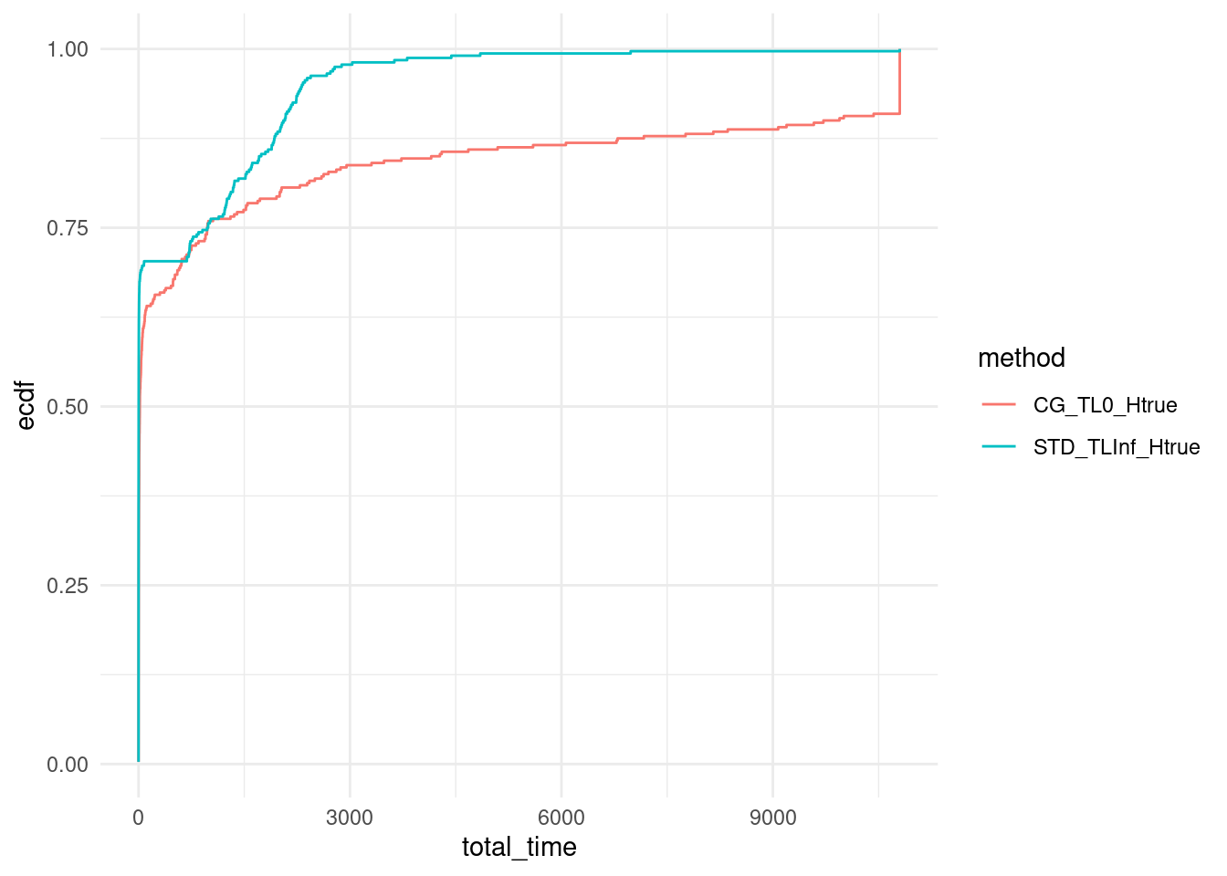
for (Gamma_val in unique(data$Gamma)) {
  print(Gamma_val)
  p = ggplot(data %>% filter(Gamma == Gamma_val), aes(x = total_time, col = method)) + stat_ecdf(pad = FALSE) +
  coord_cartesian(xlim = c(0,10800)) +
  #scale_x_log10() +
  theme_minimal()
  print(p)
}
## [1] 3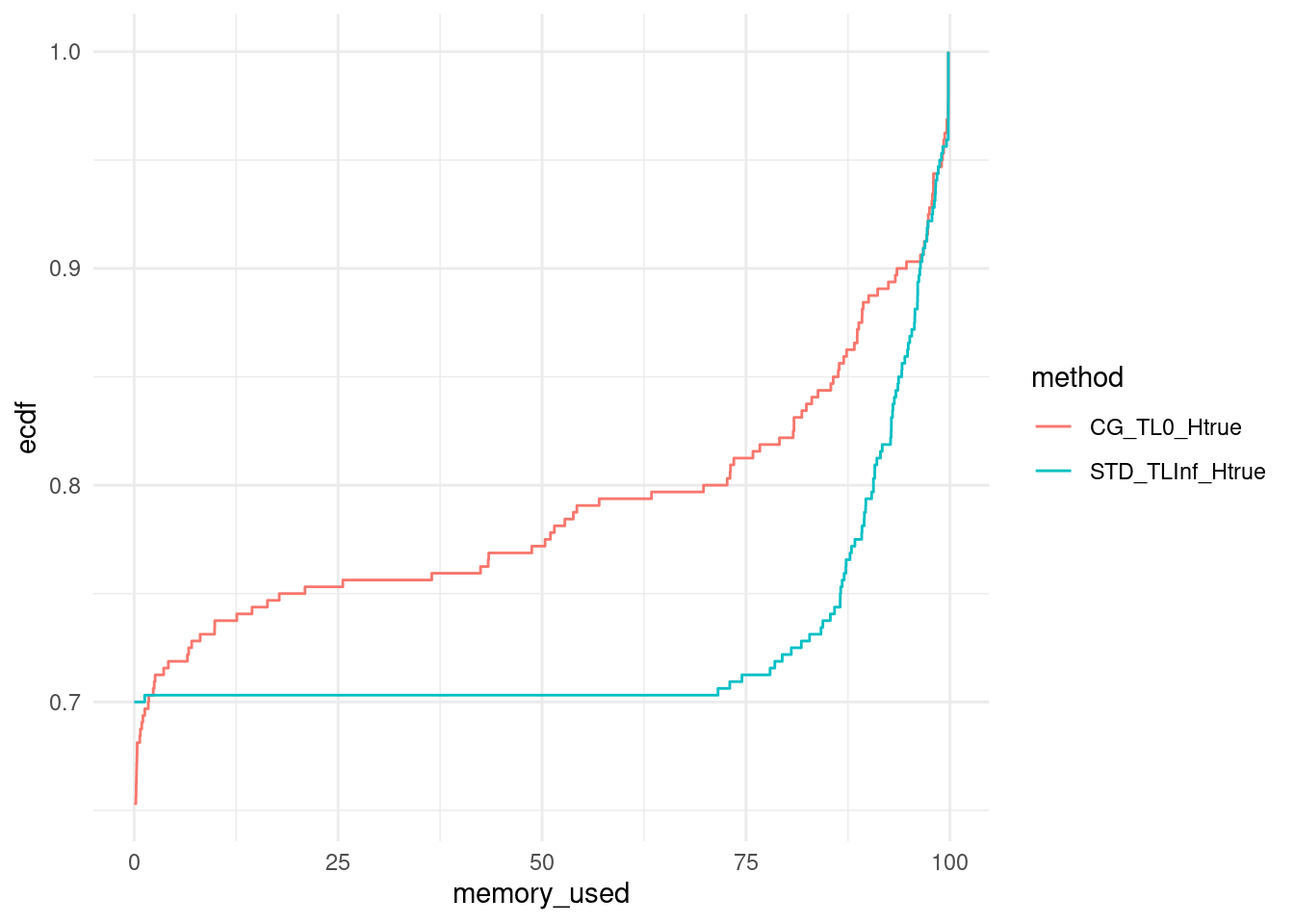
## [1] 6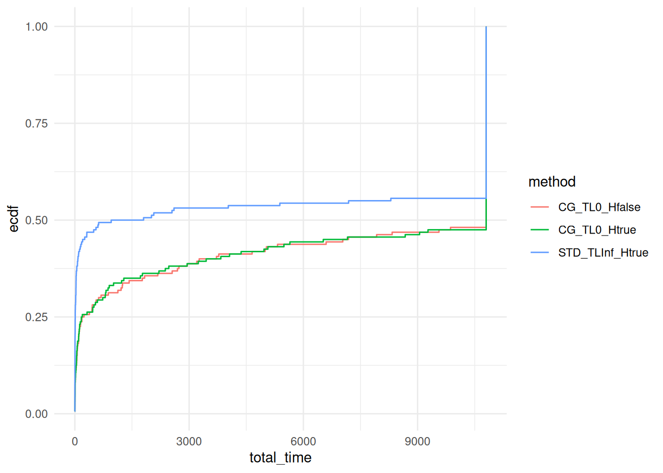
ggplot(data, aes(x = memory_used, col = method)) +
  stat_ecdf(pad = FALSE) +
  theme_minimal()
ggplot(data, aes(x = master_time / n_iterations, col = method)) + stat_ecdf(pad = FALSE) +
  # coord_cartesian(xlim = c(0,18000)) +
  theme_minimal()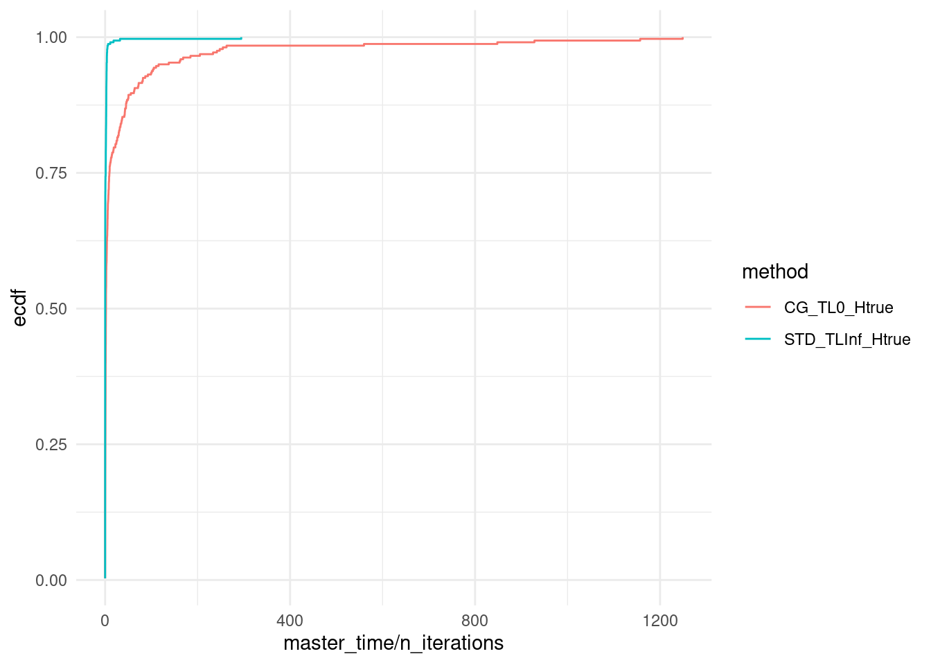
We export these results in csv to print them in tikz.
#data_with_ecdf = data %>%
#  group_by(method) %>%
#  arrange(total_time) %>%
#  mutate(ecdf_value = ecdf(total_time)(total_time)) %>%
#  ungroup()

n_points <- 1000
x_points <- seq(1, 10800, length.out = n_points)

data_with_ecdf <- data %>%
  group_by(method) %>%
  arrange(total_time) %>%
  group_modify(~ {
    # Create ECDF function for the current method
    ecdf_func <- ecdf(.x$total_time)
    # Compute ECDF values for the specified points
    tibble(total_time = x_points, ecdf_value = 100 * ecdf_func(x_points))
  }) %>%
  ungroup()

for (method in unique(data_with_ecdf$method)) {
  output = data_with_ecdf[data_with_ecdf$method == method,]
  output = output[,c("total_time", "ecdf_value")]
  output = output[output$total_time < 10800,]
  write.csv(output, file = paste0("TIME_", method, ".csv"), row.names = FALSE)
}
Summary table
In this section, we create a table summarizing the main outcome of our computational experiments.
We first focus on the solved instances.
summary_data_lt_18000 <- data %>%
  filter(total_time < 10800) %>%
  group_by(n_jobs, Gamma, method) %>%
  summarize(
    avg_total_time = mean(total_time, na.rm = TRUE),
    avg_master_time = mean(master_time, na.rm = TRUE),
    avg_adversarial_time = mean(adversarial_time, na.rm = TRUE),
    avg_n_iterations = mean(n_iterations, na.rm = TRUE),
    sum_has_large_scaled = sum(has_large_scaled),
    sum_oom = sum(tag == "iteration"),
    num_lines = n(),
    .groups = "drop"
  ) %>%
  ungroup() %>%
  arrange(n_jobs, Gamma, method)
Then, we compute averages over the unsolved instances.
summary_data_ge_18000 <- data %>%
  filter(total_time >= 10800) %>%
  group_by(n_jobs, Gamma, method) %>%
  summarize(
    avg_n_iterations_unsolved = mean(n_iterations, na.rm = TRUE),
    num_lines_unsolved = n(),
    .groups = "drop"
  ) %>%
  ungroup() %>%
  arrange(n_jobs, Gamma, method)
Finally, we merge our results.
transposed_data_lt_18000 <- summary_data_lt_18000 %>%
  pivot_wider(names_from = method, values_from = avg_total_time:num_lines)

transposed_data_ge_18000 <- summary_data_ge_18000 %>%
  pivot_wider(names_from = method, values_from = avg_n_iterations_unsolved:num_lines_unsolved)

transposed_data_lt_18000 %>% kable()| n_jobs | Gamma | avg_total_time_CG_TL0_Hfalse | avg_total_time_CG_TL0_Htrue | avg_total_time_STD_TLInf_Htrue | avg_master_time_CG_TL0_Hfalse | avg_master_time_CG_TL0_Htrue | avg_master_time_STD_TLInf_Htrue | avg_adversarial_time_CG_TL0_Hfalse | avg_adversarial_time_CG_TL0_Htrue | avg_adversarial_time_STD_TLInf_Htrue | avg_n_iterations_CG_TL0_Hfalse | avg_n_iterations_CG_TL0_Htrue | avg_n_iterations_STD_TLInf_Htrue | sum_has_large_scaled_CG_TL0_Hfalse | sum_has_large_scaled_CG_TL0_Htrue | sum_has_large_scaled_STD_TLInf_Htrue | sum_oom_CG_TL0_Hfalse | sum_oom_CG_TL0_Htrue | sum_oom_STD_TLInf_Htrue | num_lines_CG_TL0_Hfalse | num_lines_CG_TL0_Htrue | num_lines_STD_TLInf_Htrue |
|---|---|---|---|---|---|---|---|---|---|---|---|---|---|---|---|---|---|---|---|---|---|---|
| 30 | 3 | 2010.063 | 1821.504 | 158.5377 | 1986.157 | 1798.688 | 130.24936 | 23.04203 | 22.19827 | 28.20346 | 7.225807 | 7.147541 | 8.549296 | 62 | 61 | 0 | 0 | 0 | 0 | 62 | 61 | 71 |
| 30 | 6 | 1481.399 | 1394.076 | 560.3248 | 1238.982 | 1129.475 | 80.37561 | 241.80795 | 264.11766 | 479.88363 | 6.622642 | 6.673077 | 6.728814 | 53 | 52 | 0 | 0 | 0 | 0 | 53 | 52 | 59 |
| 40 | 3 | 1469.176 | 1533.361 | 315.2581 | 1438.349 | 1505.364 | 207.87783 | 29.62738 | 26.98819 | 107.23685 | 7.789474 | 7.842105 | 10.458333 | 19 | 19 | 0 | 0 | 0 | 0 | 19 | 19 | 48 |
| 40 | 6 | 1764.391 | 1471.362 | 299.4690 | 1746.922 | 1454.200 | 197.57655 | 15.00250 | 15.72054 | 101.78570 | 8.250000 | 8.291667 | 9.300000 | 24 | 24 | 0 | 0 | 0 | 0 | 24 | 24 | 30 |
transposed_data_ge_18000 %>% kable()| n_jobs | Gamma | avg_n_iterations_unsolved_CG_TL0_Hfalse | avg_n_iterations_unsolved_CG_TL0_Htrue | avg_n_iterations_unsolved_STD_TLInf_Htrue | num_lines_unsolved_CG_TL0_Hfalse | num_lines_unsolved_CG_TL0_Htrue | num_lines_unsolved_STD_TLInf_Htrue |
|---|---|---|---|---|---|---|---|
| 30 | 3 | 6.111111 | 6.473684 | 6.888889 | 18 | 19 | 9 |
| 30 | 6 | 6.111111 | 5.964286 | 8.571429 | 27 | 28 | 21 |
| 40 | 3 | 5.672131 | 5.786885 | 8.906250 | 61 | 61 | 32 |
| 40 | 6 | 3.821429 | 3.892857 | 6.500000 | 56 | 56 | 50 |
#cbind(
#  transposed_data_lt_18000,
#  transposed_data_ge_18000
#) %>%
#  kable() %>%
#  kable_styling(full_width = FALSE, position = "center")
Second-stage Deviations
ggplot(data, aes(x = method, y = second_stage.std_dev / abs(second_stage.mean))) +
  geom_boxplot() +
  labs(title = "Boxplot of std.dev",
       x = "Method",
       y = "Number of Iterations") +
  theme_minimal()
## Warning: Removed 960 rows containing non-finite outside the scale range
## (`stat_boxplot()`).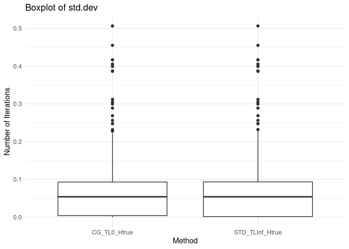
git push action on the public repository
hlefebvr/hlefebvr.github.io using rmarkdown and Github
Actions. This ensures the reproducibility of our data manipulation. The
last compilation was performed on the 05/03/26 11:03:36.