Table of Contents
Statistics on Bruxelles Marathon (2023)
We used the data set from the official Brussels Marathon website provided by ACN-timing. Raw results in XML format can be accessed here. Then, we preprocessed the data to convert it into a csv file. No data was removed.
data = read.csv("results.csv", header = FALSE)
colnames(data) = c("rank", "bib", "name", "nat_flag", "10km_time_in_ms", "21_1km_time_in_ms", "30km_time_in_ms", "checkpoint", "time", "estimation", "avg", "category_rank", "category")
Cleaning the data
First, we add a column for gender.
data$gender <- ifelse(substr(data$category, 1, 1) == "F", "female", "male")The data set has ranks as strings with trailing points. We make them integers.
data$rank = as.integer(data$rank)## Warning: NAs introduced by coercionLooking at the official results, people with ranking greater than 1420 have missing entries and strange finish times (e.g., below world record). We eliminate these rows (20 rows).
data = data[data$rank < 1420,]We also clean the data according to the following filter.
filter = data$rank == "DSQ" | is.na(data$rank) | is.na(data$time) | data$time == ""

data = data[!filter,]
Finally, we convert the given times into seconds so that statistics can be easily computed.
# Convert the TIME column to POSIXlt
data$time_posix = as.POSIXlt(data$time, format = "%H:%M:%S")

# Extract hours, minutes, and seconds
data$hours = data$time_posix$hour
data$minutes = data$time_posix$min
data$seconds = data$time_posix$sec

# Calculate total time in seconds
data$time_seconds = data$hours * 3600 + data$minutes * 60 + data$secondsHistogram of finish times
# Create a histogram of TIME_S
ggplot(data, aes(x = time_seconds)) +
  geom_histogram(binwidth = 60, fill = "blue", color = "blue") + # binwidth in seconds
  labs(
    title = "Distribution of TIME_S",
    x = "Time in Seconds",
    y = "Frequency"
  ) +
  scale_x_continuous(
    breaks = seq(0, max(data$time_seconds), by = 3600), # Label every hour
    labels = function(x) {
      h <- floor(x / 3600)
      m <- floor((x %% 3600) / 60)
      s <- x %% 60
      sprintf("%02d:%02d:%02d", h, m, s)
    }
  )+
  facet_grid(. ~ gender)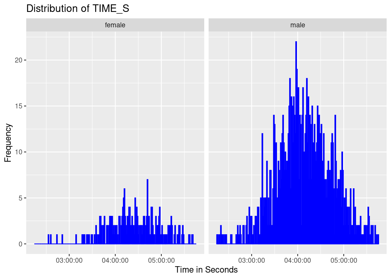
Empirical Cumulative Distribution Function (ECDF)
major_breaks <- seq(0, 21600, by = 60 * 60 / 2) # Major ticks every hour
minor_breaks <- seq(0, 21600, by = 5 * 60)  # Minor ticks every 10 minutes

# Create an ECDF plot of TIME_S with formatted x-axis labels
ggplot(data, aes(x = time_seconds, color = gender)) +
  geom_step(stat = "ecdf") +
  labs(
    title = "ECDF of TIME_S",
    x = "Time (H:M:S)",
    y = "Cumulative Probability"
  ) +
  scale_x_continuous(
    breaks = major_breaks,
    minor_breaks = minor_breaks,
    labels = function(x) {
      h <- floor(x / 3600)
      m <- floor((x %% 3600) / 60)
      sprintf("%02d:%02d", h, m)
    }
  ) +
  scale_y_continuous(
    breaks = seq(0, 1, by = .1)
  ) +
coord_cartesian(xlim = c(2.4 * 3600, 6 * 3600)) 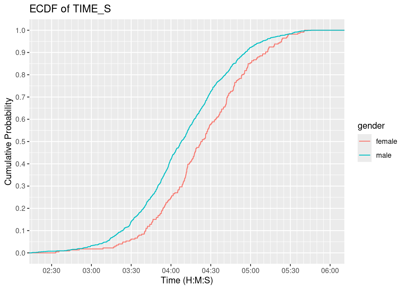
# Convert time_seconds to ECDF for each gender
ecdf_male <- ecdf(data[data$gender == "male",]$time_seconds)
ecdf_female <- ecdf(data[data$gender == "female",]$time_seconds)

# Create a sequence of probability values from 0 to 1
times <- seq(2 * 3600 + 15 * 60, max(data[data$gender == "male",]$time_seconds), by = 5 * 60)  # Adjust the step as needed
times_str <- sprintf("%02d:%02d:00", times %/% 3600, (times %% 3600) %/% 60)

# Create a data frame with ECDF values for each gender
ecdf_table <- data.frame(
  times = times_str,
  male = ecdf_male(times) * 100,
  female = ecdf_female(times) * 100
)

knitr::kable(ecdf_table,
               digits = c(0, 2, 2),
               col.names = c("Time", "Male", "Female")
             ) %>%
kable_classic()| Time | Male | Female |
|---|---|---|
| 02:15:00 | 0.08 | 0.00 |
| 02:20:00 | 0.34 | 0.00 |
| 02:25:00 | 0.59 | 0.00 |
| 02:30:00 | 0.75 | 0.00 |
| 02:35:00 | 0.92 | 0.44 |
| 02:40:00 | 1.01 | 0.88 |
| 02:45:00 | 1.42 | 1.33 |
| 02:50:00 | 1.93 | 1.33 |
| 02:55:00 | 2.35 | 1.77 |
| 03:00:00 | 3.27 | 1.77 |
| 03:05:00 | 3.69 | 1.77 |
| 03:10:00 | 4.78 | 2.21 |
| 03:15:00 | 6.79 | 2.21 |
| 03:20:00 | 8.80 | 3.54 |
| 03:25:00 | 11.15 | 4.87 |
| 03:30:00 | 14.08 | 6.19 |
| 03:35:00 | 17.10 | 7.52 |
| 03:40:00 | 20.54 | 8.85 |
| 03:45:00 | 24.98 | 12.83 |
| 03:50:00 | 29.67 | 15.93 |
| 03:55:00 | 35.37 | 20.80 |
| 04:00:00 | 41.99 | 24.78 |
| 04:05:00 | 47.11 | 26.99 |
| 04:10:00 | 51.72 | 32.30 |
| 04:15:00 | 57.42 | 41.15 |
| 04:20:00 | 62.03 | 47.35 |
| 04:25:00 | 66.55 | 51.33 |
| 04:30:00 | 72.51 | 57.52 |
| 04:35:00 | 76.78 | 61.06 |
| 04:40:00 | 79.46 | 65.49 |
| 04:45:00 | 83.32 | 72.12 |
| 04:50:00 | 86.59 | 77.43 |
| 04:55:00 | 89.35 | 80.09 |
| 05:00:00 | 92.29 | 85.40 |
| 05:05:00 | 94.13 | 87.61 |
| 05:10:00 | 95.31 | 89.38 |
| 05:15:00 | 96.40 | 92.48 |
| 05:20:00 | 97.23 | 93.81 |
| 05:25:00 | 97.74 | 96.46 |
| 05:30:00 | 98.41 | 98.23 |
| 05:35:00 | 99.16 | 98.23 |
| 05:40:00 | 99.66 | 99.12 |
| 05:45:00 | 99.92 | 100.00 |
This document is automatically generated after every
git push action on the public repository
hlefebvr/hlefebvr.github.io using rmarkdown and Github
Actions. This ensures the reproducibility of our data manipulation. The
last compilation was performed on the 04/03/25 16:25:53.